Small example of using PyTorch Lightning with PBS

  
#!/bin/bash

## Required PBS Directives --------------------------------------
#PBS -A <account>
#PBS -q <queue>
#PBS -l select=4:ncpus=40:mpiprocs=1:nmlas=2
#PBS -l walltime=24:00:00

# Configure Cluster
export MASTER_PORT=8148
NODES=$(cat $PBS_NODEFILE | sort | uniq)
MASTER_ADDR=$(echo $NODES | cut -d ' ' -f 1)
export WORLD_SIZE=$(wc -l < $PBS_NODEFILE) 

# Debugging flags
export NCCL_P2P_DISABLE=0
export NCCL_DEBUG=WARN

echo "  MASTER_ADDR is: $MASTER_ADDR"
echo "  MASTER_PORT is: $MASTER_PORT"
echo "  WORLD_SIZE is : $WORLD_SIZE"

# Loop through all nodes and start the training.
NODE_RANK=0
for NODE in $NODES; do
    echo "Starting training on $NODE with NODE_RANK $NODE_RANK, MASTER_ADDR $MASTER_ADDR, MASTER_PORT $MASTER_PORT"
    # Ensure no spaces after the backslash ending each line.
    ssh $NODE "bash; \
        export MASTER_ADDR=$MASTER_ADDR; \
        export MASTER_PORT=$MASTER_PORT; \
        export WORLD_SIZE=$WORLD_SIZE; \
        export NODE_RANK=$NODE_RANK; \
        source ~/miniconda3/bin/activate <your env>; \
        cd <your dir> \
        echo \"   On $NODE_RANK with NODE_RANK $NODE_RANK, MASTER_ADDR $MASTER_ADDR, MASTER_PORT $MASTER_PORT, WORLD_SIZE $WORLD_SIZE\"; \
        python your_code.py fit --config configs/your_yaml.yaml --trainer.strategy=ddp --trainer.num_nodes=$WORLD_SIZE; \
    " &
    NODE_RANK=$((NODE_RANK + 1))
done

# Wait for all child processes to complete.
wait

This script fetches the node information from PBS. This information is only available on the master node. Next, it ssh’s into each node in the cluster allocated to your job, sets the appropriate environment variables (these tell Pytorch lightning how to communicate with the master node), and then launches your training script. The master node is automatically set when you set its environment variable, NODE_RANK = 0.

I left in the NCCL debugging flags which are helpful in debugging when the script hangs or nodes can’t communicate to each other. These can be easily commented out.

NES Castlevania II Cheat Code

CTMVW26KR5KNSIBK

I don’t know why I still know this 30 years after learning it.

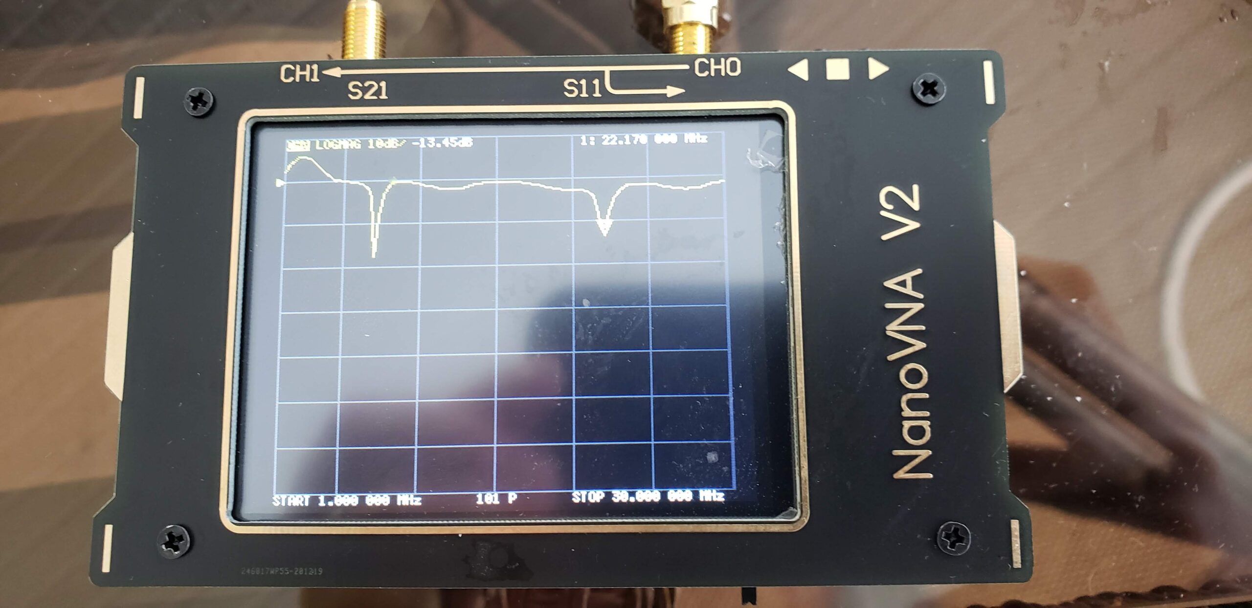
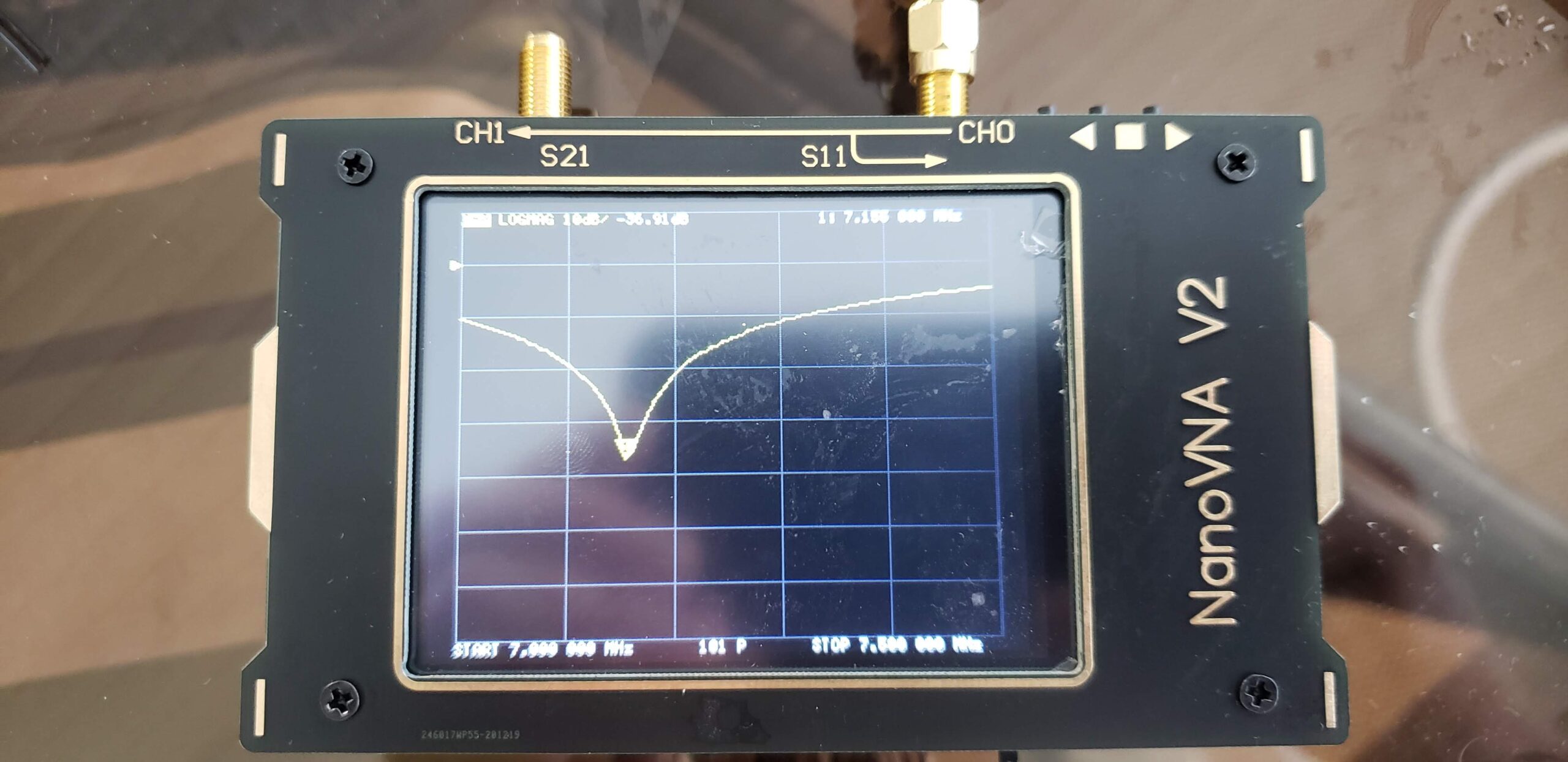
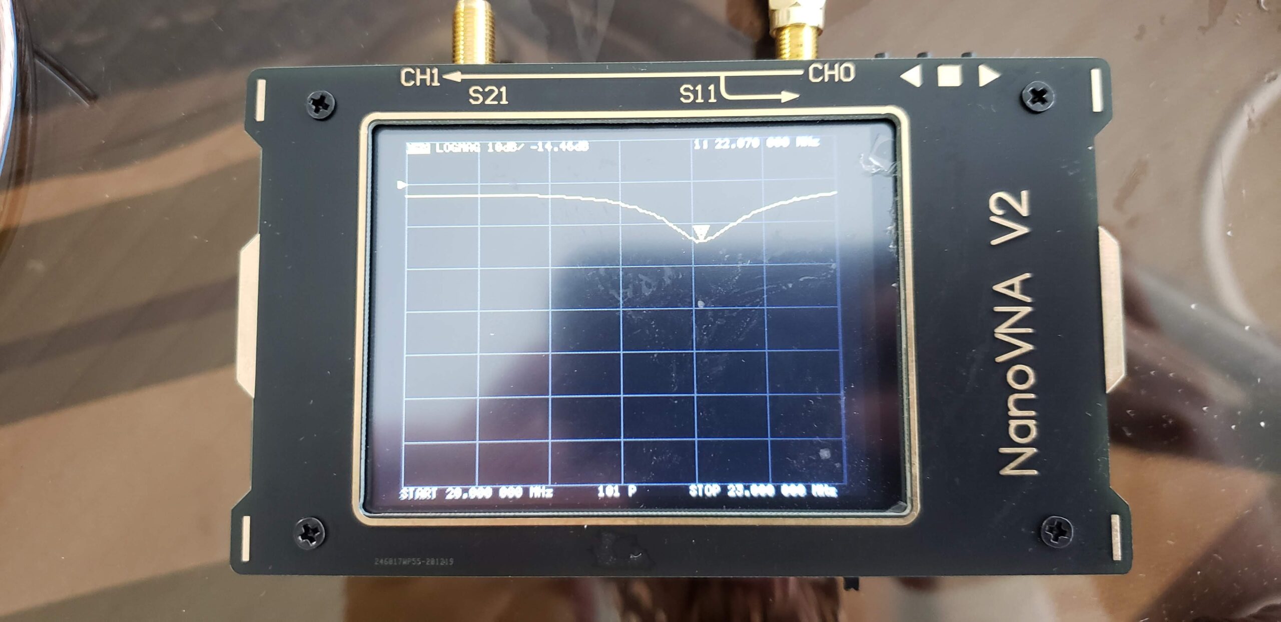
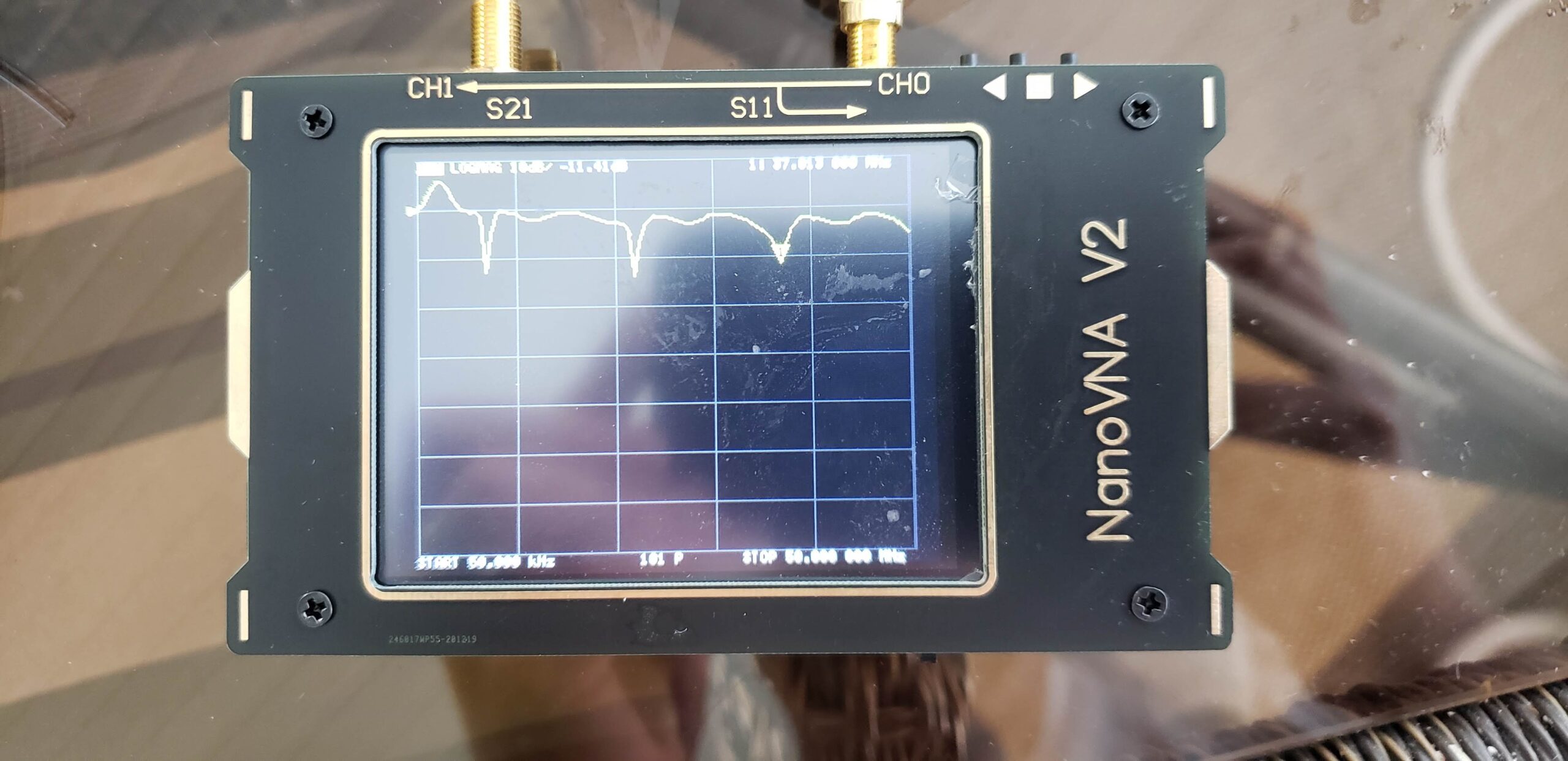
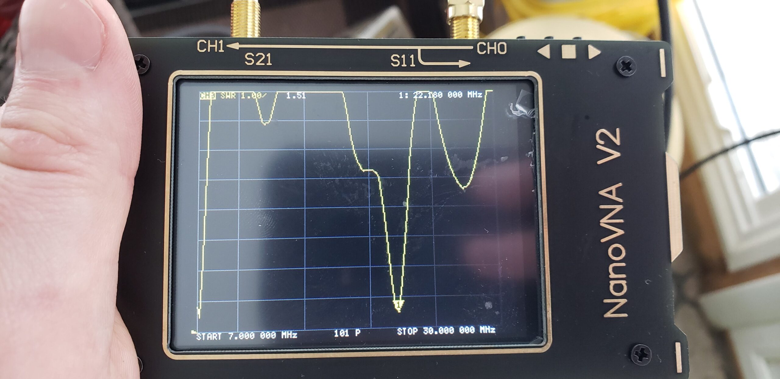
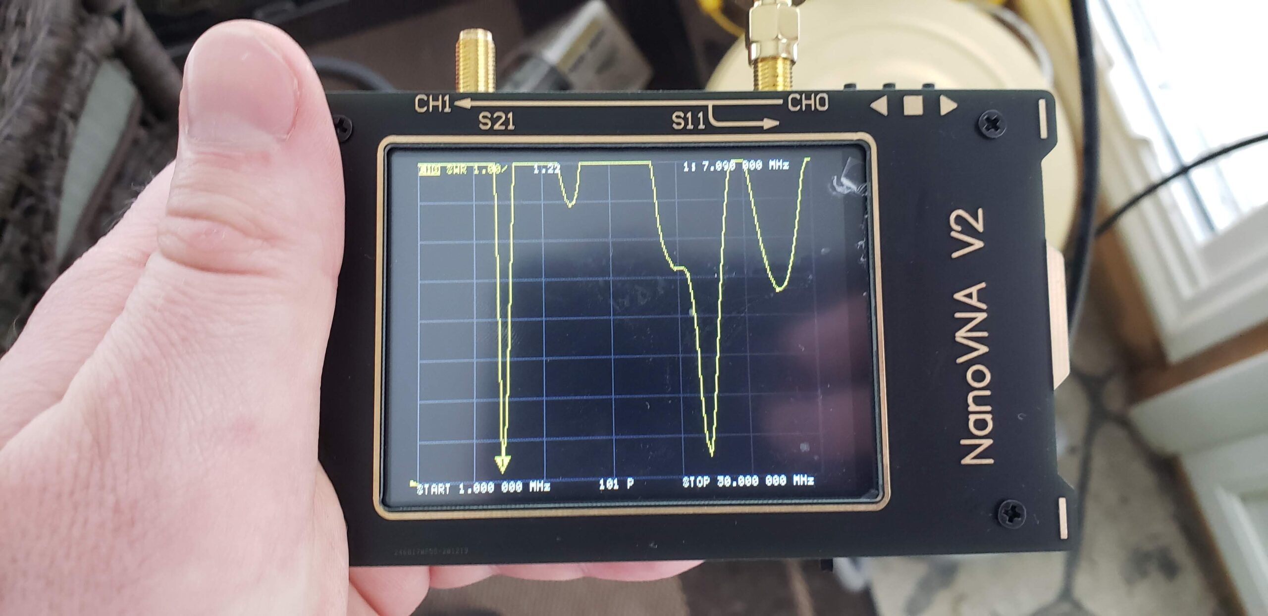
Dipole Antenna Measurements

1 to 30MHz log mag, marker at 22.170MHz.

7 – 7.5 MHz, Marker at 7.155 MHz

20-23MHz,marker at 22.070MHz

50kHz – 50MHz, marker at 37.013MHz


7-30MHz, SWR, marker at 22.180MHz

1-30MHz, SWR, marker at 7.090MHz

Tensorboard subsamples scalars when plotting

I have noticed for year that tensorboard v2.x subscamples scalars when plotting.  I never tried to reproduce the problem but noticed if I had a longish training run, every epoch’s loss was not displayed on tensorboard.  This would produce a strange jaggy effect of the plot which I never liked, especially given my signal processing background.  It was also not obvious why or how it was subsampling.  For all I knew, it wasn’t even subsampling but doing some kind of filtering which resulted in the skipping of scalar values on the plots.

Today, I finally figured out how to fix this issue.  I was able to correct the issue by using a tensorboard command prompt of:

start “tensorboard” “e:\python_3.8\scripts\tensorboard” –samples_per_plugin scalars=9999999 –logdir .

The addition of the –samples_per_plugin scalars=999999 fixes the issue.  Now, all of the points I write out to tensorboard are displayed.

Ref: https://stackoverflow.com/questions/43763858/change-images-slider-step-in-tensorboard

GOES Satellite Downlink Capture

This video is from the GOES Satellite imaging sensor over a 24 hour period.

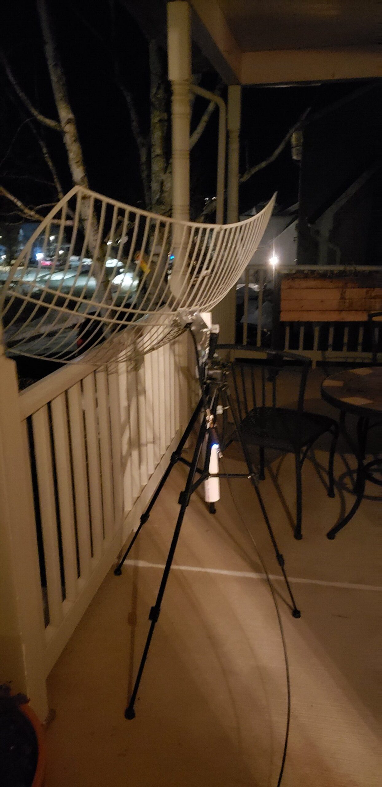
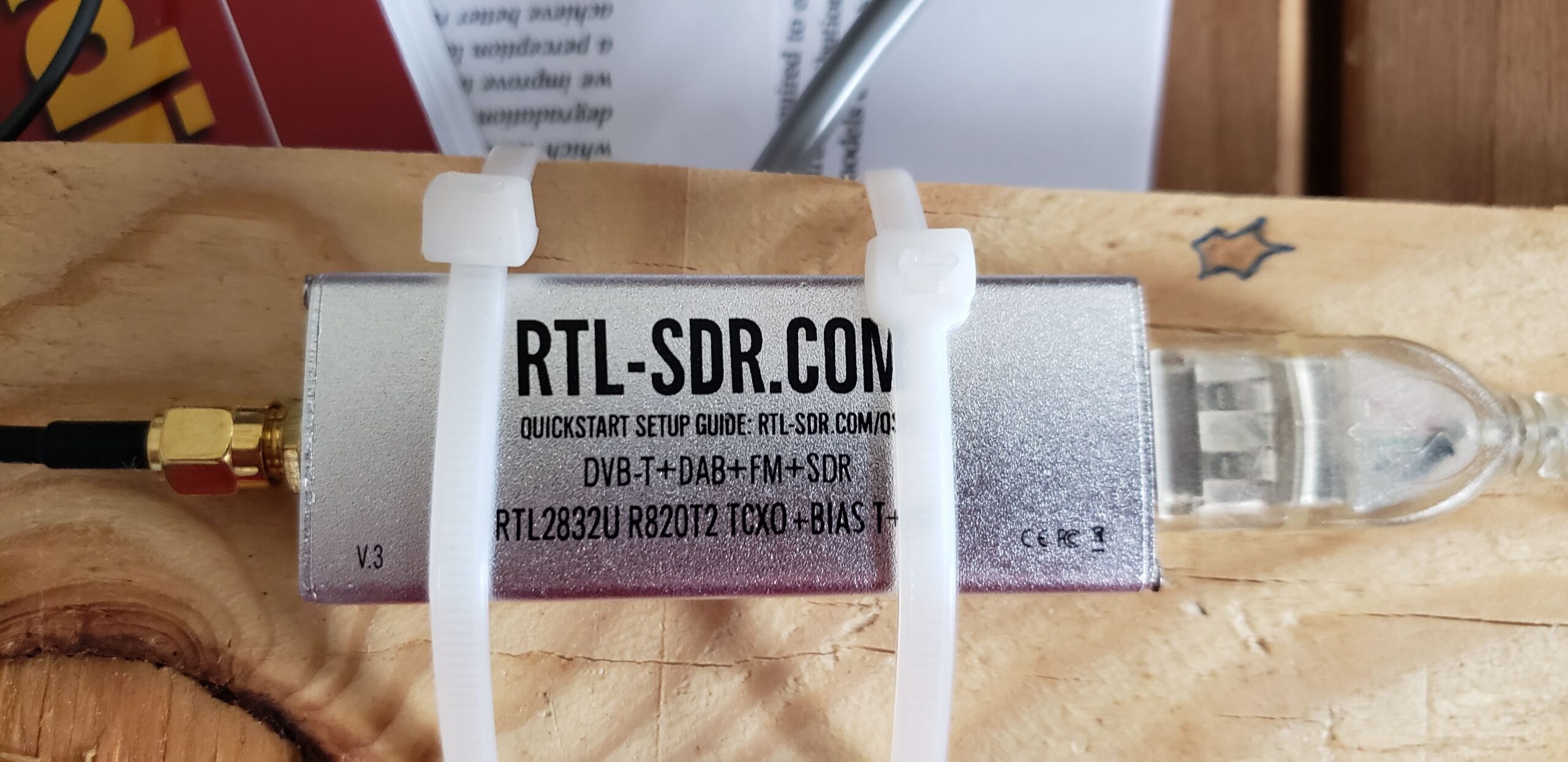
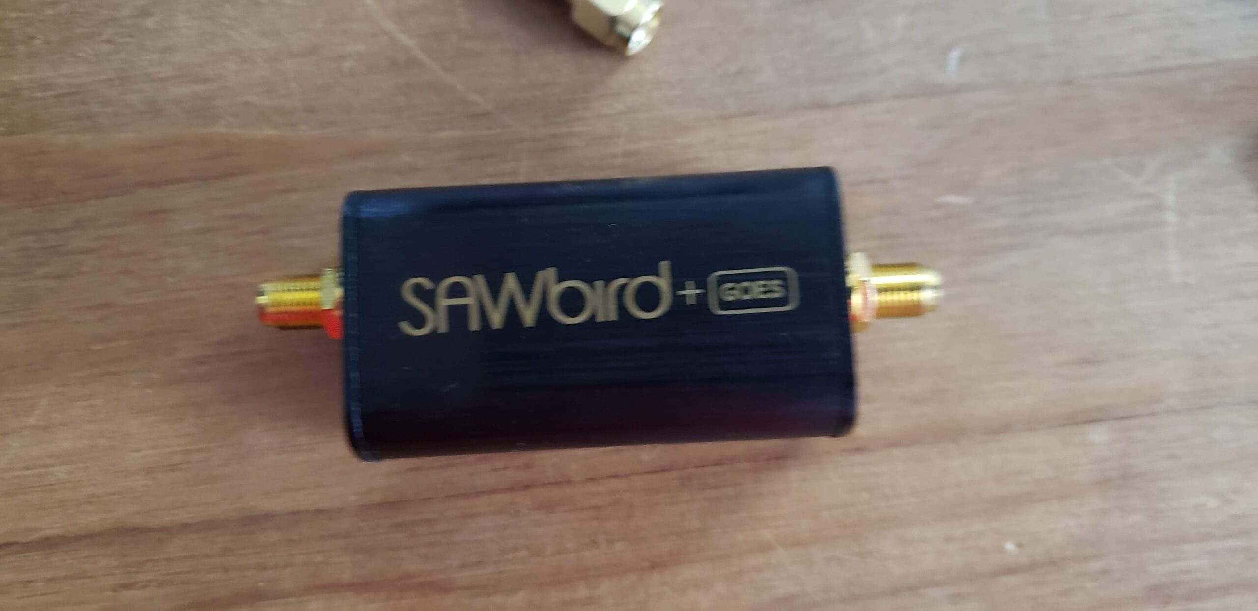
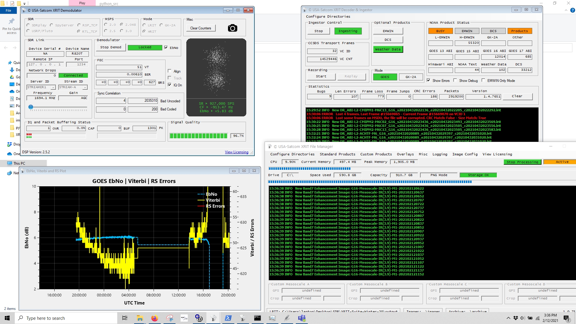
I captured this using a SawBird LNA, a WiFi dish, an RTL-SDR, and the XRIT decoding software.


Screenshot of the “groundstation terminal.”

Source code to compile the video is below.

import os
import glob

import cv2
import matplotlib.pyplot as plt
import numpy as np
import tqdm

data_dir = r'C:\Users\laptop\Desktop\SDR\XRIT-Suite-Winter-20\images'
files = sorted(glob.glob(os.path.join(data_dir, '*full*fsclr*.png')), key=os.path.getmtime) # full disk
files = files[53:53+48+2]
N = len(files)

# Make mask
img = cv2.imread(os.path.join(data_dir, 'G16-Full Disk-FSCLR-202102101800.png'))
mask = np.mean(img, axis=2) == 0
mask[:162,:] = 0 
mask[5617:,:] = 0
mask = (~mask.astype('bool')).astype('uint8')

images = np.zeros((N, 5961//2, 5424//2, 3), dtype='uint8')
for fidx, f in enumerate(files):
   #img = cv2.cvtColor(cv2.imread(f), cv2.COLOR_BGR2RGB)
   img = cv2.imread(f) 
   if img.shape[0] != 5961:
      continue
   # Post process
   img = cv2.medianBlur(img, 7)
   img = img*mask[:,:,None]

   img = cv2.resize(img, (0,0), fx=0.5, fy=0.5, interpolation=cv2.INTER_AREA)
   images[fidx,:,:,:,] = img

fourcc = cv2.VideoWriter_fourcc(*'MJPG')
out = cv2.VideoWriter('output.avi',fourcc, 30, (5424//2, 5961//2))
for k in tqdm.tqdm(np.linspace(0,N-2,N*15)):
   f = int(np.floor(k))
   offset = k - f
   print(offset)
   frame = ((1-offset)*images[f,:,:,:].astype('float32') + offset*images[f+1,:,:,:].astype('float32')).astype('uint8')
   out.write(frame)

out.release()
print('done')

Cryptic Numba Error – Use Parentheses for numpy.array, Not Brackets

I am writing a fairly complicated Numba code and kept getting a cryptic error which took me a few hours to figure out.  The error was the following:

numba.core.errors.TypingError: Failed in nopython mode pipeline (step: nopython frontend)
No implementation of function Function(<built-in function array>) found for signature:
>>> array(array(float64, 1d, C))
There are 2 candidate implementations:
- Of which 2 did not match due to:
Overload in function 'array': File: numba/core/typing/npydecl.py: Line 504.
With argument(s): '(array(float64, 1d, C))':
Rejected as the implementation raised a specific error:
... (truncated)

I discovered that the problem was the result of creating new numpy arrays using lists instead of tuples.  So instead of np.array([1,2,3]), I was supposed to do np.array((1,2,3)).  That’s it!

I found the solution by reading the Numba documentation (https://numba.pydata.org/numba-doc/latest/reference/numpysupported.html)

(nested lists are not yet supported by Numba)

Converting Mag and Phase to Real and Imaginary in Tensorflow 2 on Windows 10

As of Tensorflow 2.1, you cannot do the following when running in a windows 10 environment on the GPU (it does work fine if you are running on the CPU though):

r = tf.complex(magnitude, 0.0) * tf.math.exp(tf.complex(0.0,1.0)*tf.complex(phase, 0.0))

This results in a barrage of “CUDA_ERROR_LAUNCH_FAILED: unspecified launch failure” error messages. I filed a bug report here: https://github.com/tensorflow/tensorflow/issues/38443

You can see from the tensorflow code, I am doing a simple operation: converting the magnitude and phase representation of a complex number into real and imaginary representation. I am doing this by utilizing the phase rotation properties of the exponential function (i.e. e^{i phase}).

I did come up with a workaround which I am posting here to prevent someone else spending hours of their time on a similar error, questioning their judgement, and thinking this should trivially work. My workaround converts magnitude and phase to real and imaginary through Euler’s formula.

def mag_phase_2_real_imag(mag, phase):      
    cos_phase = tf.math.cos(phase)
    sin_phase = tf.math.sin(phase)
    r= tf.complex(mag*cos_phase, mag*sin_phase)
    return  r
#    

real_imag = tf.keras.layers.Lambda(lambda x:mag_phase_2_real_imag(x[0], x[1]))([mag, phase])  

[Talk] Beyond Empirical Risk Minimization: the lessons of deep learning

Some of Our Favorite Rides in State College

List of Italy Posts

http://www.gergltd.com/home/2018/04/welcome-to-italy/

http://www.gergltd.com/home/2018/04/pictures-from-italy/

http://www.gergltd.com/home/2018/04/mountain-biking-in-lerici-italy/

http://www.gergltd.com/home/2018/04/more-pictures-of-the-ruins-in-redarca/

http://www.gergltd.com/home/2018/05/our-visit-to-the-carrara-marble-mines/

http://www.gergltd.com/home/2018/06/some-of-our-favorite-views-on-our-mountain-bike-rides/


Some of Our Favorite Views on Our Mountain Bike Rides

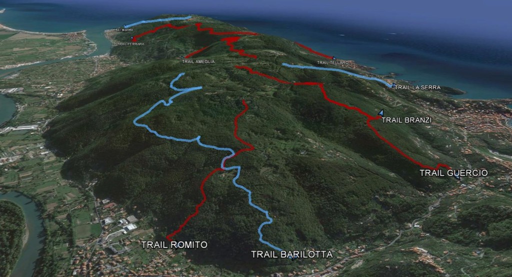
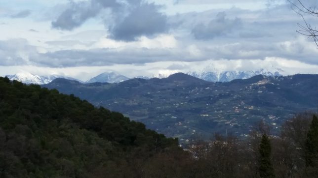
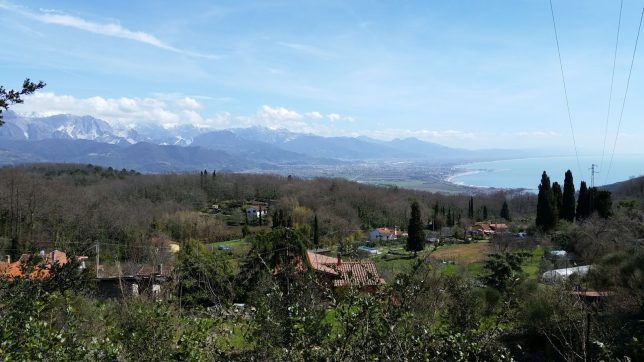
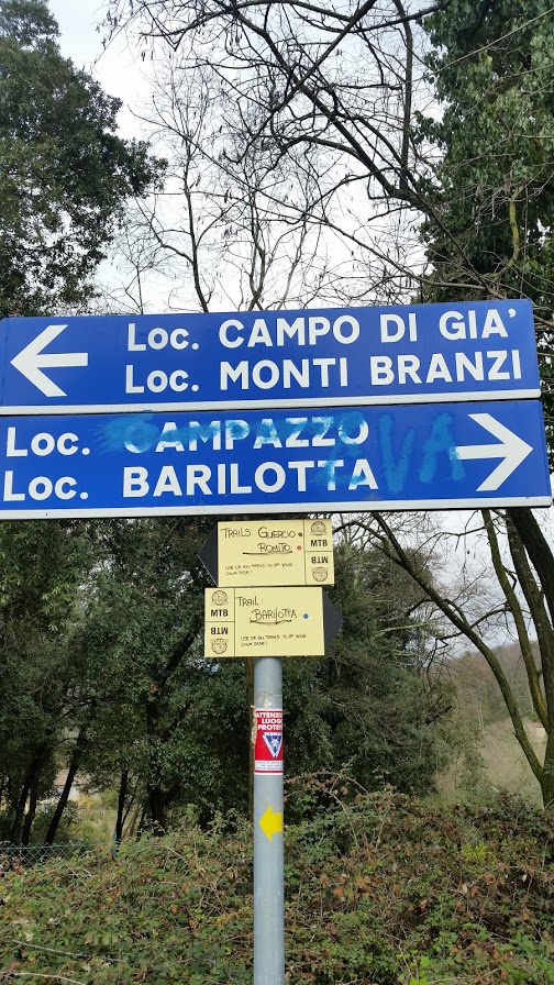
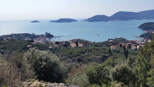
We mountain bike quite a bit in Redarca, a little village behind Lerici, Italy. The trails are well maintained and mostly enduro types. I spend most of my time biking the trails around Monte Branzi and the surrounding area (Snake, Guercio, Branzi, Buck).

[momentopress url=https://momento360.com/e/u/1dc752ffe44e4088bac5c69df08b7a54?utm_campaign=embed&utm_source=other&utm_medium=other]

[momentopress url=https://momento360.com/e/u/ece1d6654dd74321be4be096ff559ef0?utm_campaign=embed&utm_source=other&utm_medium=other]

[momentopress url=https://momento360.com/e/u/eec5905447944bcaab74b415f3b48087?utm_campaign=embed&utm_source=other&utm_medium=other]

[momentopress url=https://momento360.com/e/u/a3b58bac643240148e611304e89a8c2c?utm_campaign=embed&utm_source=other&utm_medium=other]

Google Earth view of some of our favorite trails.

Photo courtesy of http://www.lericibike.com/2016/05/16/trail-branzi-2-2km/

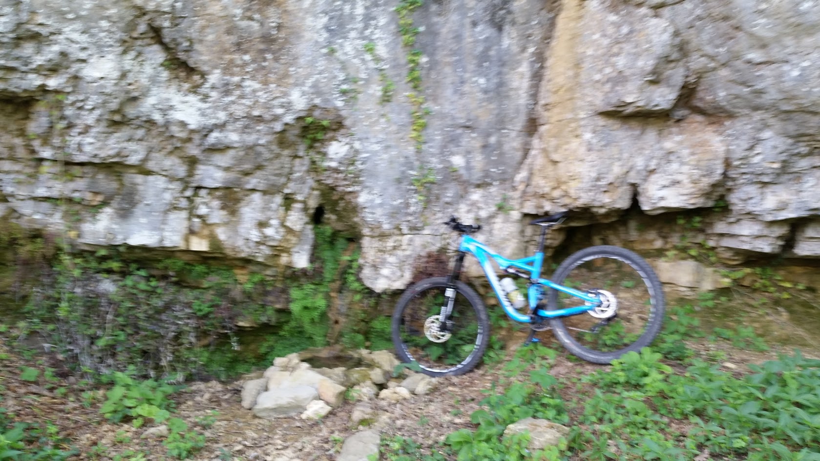
Blurry shot of the Peocio fountain (peace fountain).

Our Visit to the Carrara Marble Mines

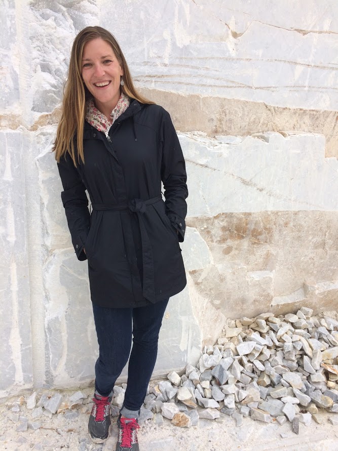
We took a tour through the Carrara Marble Mines.  If you’re a James Bond fan, you’ve likely had already seen them.  The opening scene of Quantum of Solace was filmed here.  We drove the same roads as James Bond and even visited the house the car crashes into before going over the cliff.  Can you spot the similarities in our photos below?
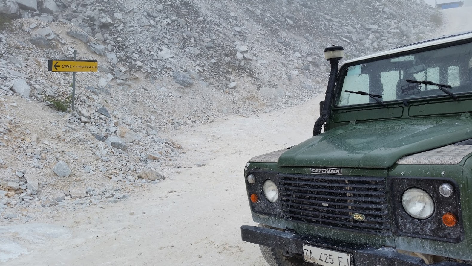
When you see the white peaks of the mountains in this post, its all marble, not snow!

Carrera has been mined for its marble since Roman times.    As our guide said, “It’s not money-making or a product, marble is our culture.” Everywhere you look in the town, you will see its marble. The use of it was never meant for show, it was simply a sturdy building material that was local and abundantly available.

We were greeted at the Carrara-Avenza trail station by our guide Gabrielle.  He picked us up, along with 2 other Americans, in a Land Rover Defender.  It arrived with white marble-covered tires entirely cloaked in a pale, light dusting of the stuff.  After buckling up in the Rover, Ryanne spotted a sticker on the windshield which read, “It’s not a jeep, it’s a f**king Land Rover.”  The tour we signed up for mentioned it would be taking us deep into the quarries and by all indications, we knew they weren’t kidding.

Everything you see in the Carrara mountains is marble.  There is no granite, no sandstone, no limestone; just marble.  The marble gets colored from impurities and oxidation just like any other mineral, but everywhere you look, marble. All the vegetation you see; growing in the cracks of the marble. No soil whatsoever.  All the minerals for the plants come from the marble as does the water which pools in cracks of the stone.

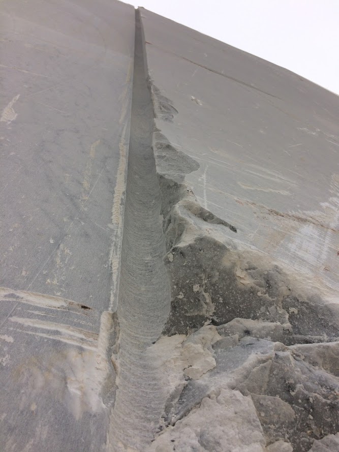
As we slowly inch our way up the steep roads of the quarry, you see massive blocks of marble.  Many the size of an American SUV and some even bigger.  The marble is mined from the outside in on the mountain.  Why dig for the marble when it’s everywhere, including the surface?  The marble is mined by cutting it into large blocks and then shipping the blocks.  A typical block is cut from the mountain-side by first drilling 3 holes into the earth: one vertical and two horizontal which all intersect.  Now, a special kind of saw is brought in to begin cutting away the block from the mountain.  The “saw” is really a rope which is threaded between 2 of the holes.  The “saw” cuts the block by cycling the rope through these holes with the friction of the rope cutting into the earth.  After 3 cuts are made, the block is free.
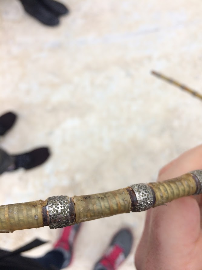
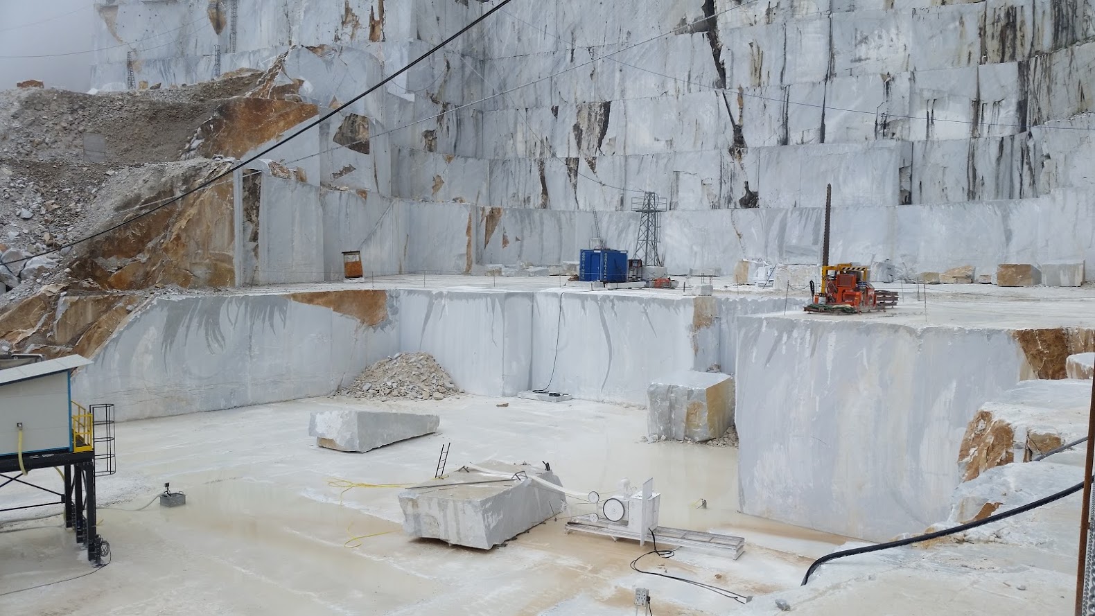
The rope I mentioned is no ordinary rope, but one made from a steel cable with bits of diamond on the outside giving it sharp teeth to cut.  As the saw cuts into the earth, it is pulled back from the mountain on rails as to keep the rope tight against the earth to make the cut.

Driving in the Marble quarry is serious business.  The roads are steep and windy like hairpins. At one point, our guide had to drive up the mountain backward for traction to get us to the next destination.  Definitely not a tour for those afraid of heights.  Ryanne took a great video while we were climbing one of the roads in the Land Rover to show the effect. On the drive back down the mountain, no one was saying a word. The driver asked, quite cheeky, why we were so quiet. We told him we wanted to make sure he would have no distractions and be fully focused!

Looking at the marble in the quarries brings mixed emotions.  On one hand, it’s amazing to see all the engineering man has been able to create. The sheer size of the equipment, the ingenuity of the design, the ability of to “tame the mountain,” and the beauty of the marble are all a wonder.  On the other hand, its a shame to think what man is doing to this natural beauty by slowing carving away at it for the sake of countertops, buildings, and cosmetic products; all things for which the marble is used.

Walking around the quarry is pretty amazing though.  Seeing your footprints on the ground in the white dust makes you think of the astronaut’s footprints on the moon.  All the mud puddles you see have a white-turquoise tint from the marble dust — reminds me of moon milk inside underground caves.

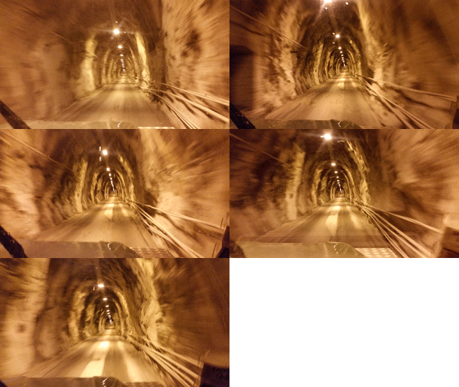
There are many digging sites at the quarry, most exposed to the surface.  However, there are a few sites which do go into the mountain.  All the quarry sites are numbered and our tour consisted of driving from site to site from the front side of the mountain to the back and then through a tunnel back to our starting point.  Quite an experience!

Ciao!


[envira-gallery id=”930″]

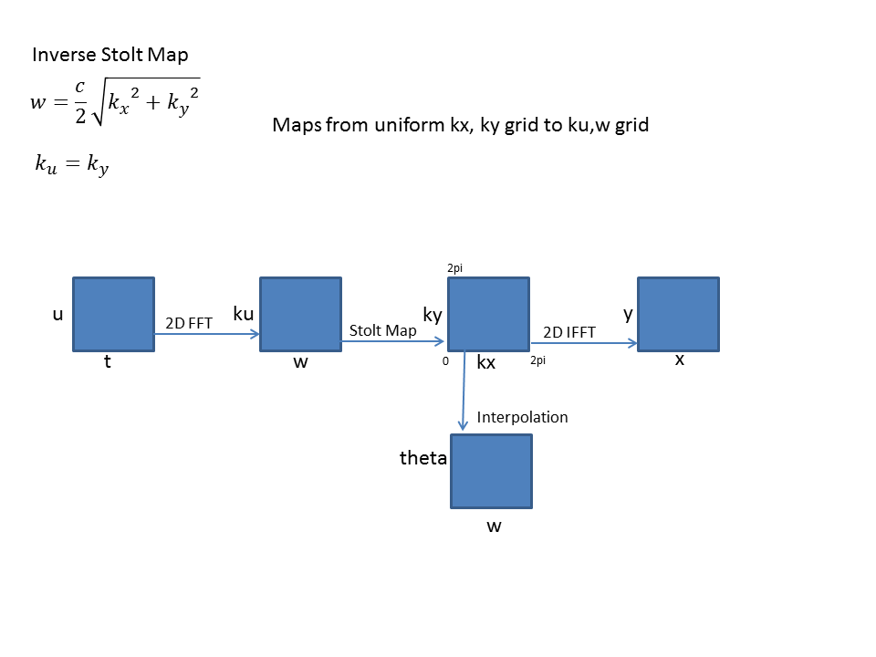
Stolt Map Notes for SAS

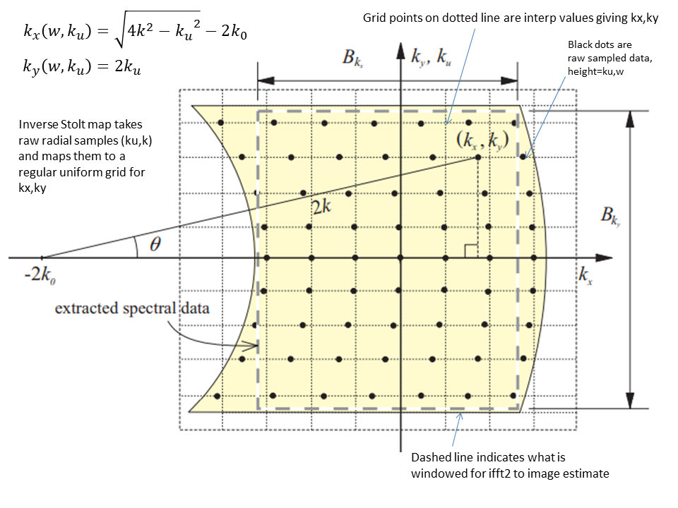
Figure adapted from Hawkins. Synthetic Aperture Imaging Algorithms:with application to wide bandwidth sonar.Phd Thesis. 1996. https://ir.canterbury.ac.nz/bitstream/handle/10092/1082/thesis_fulltext.pdf?sequence=1&isAllowed=y


More Pictures of the Ruins in Redarca

Yesterday I blogged about the 17th-century ruins off of a mountain bike trail in Redarca.  I took Ryanne there this evening to see them.  She took some really great pics including some nice ones of the frescoes.  I wanted to share so here they are.

[envira-gallery id=”881″]

Mountain Biking in Lerici Italy

There’s a reasonable amount of mountain biking here in Lerici.  It’s not nearly as big as Rothrock, but it still beautiful and worth putting in the effort to see.  We bike in areas behind our flat called Monte Rochetta and Redarca.  It’s a 3-mile uphill ride to get to the trailheads.  There are quite a few gravel roads but most of the true mountain biking trails are enduro style quite so because it’s very hilly around here.  Many of the trails are built for a single direction of travel. Everything is well labeled though with the trail name and its difficulty level (they use the green, blue, black diamond system).  Many of the true MTB trails here are black diamonds.

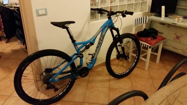
I picked up a whip from a place called Eurobike in Romita Magra.  It’s a 2015 Specialized Stumpjumper Comp Evo (aluminum).  Slightly different feel from my Salsa Horsethief and El Mariachi back home.  I also rarely ride Specialized bikes.  I like the bike well enough though.  I ride 27.5″ wheels here with tubes which were recommended by the store owner given the terrain.  At home, I have been running 29″ wheels tubeless for as far as I can remember; that was a bit of a change for me.  The guy who sold me the bike was great.  He even dropped it off for me because I couldn’t take it on the bus.  In fact, we bought Ryanne’s bike (the yellow one in the pics below) from there as well.  Again, the guy offered to take the to our flat free of charge.  While we were waiting for the bus from Eurobikes to head home, we ran into the same guy and he stopped and let us hitch a ride home with him!

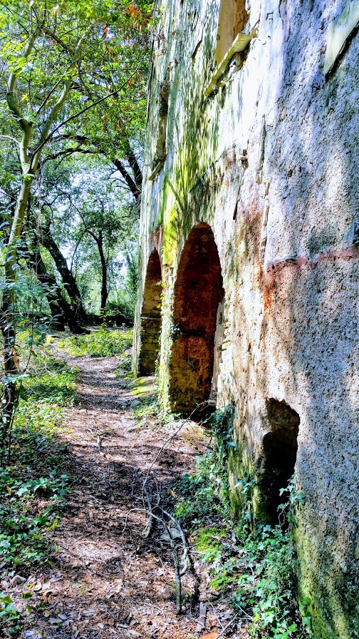
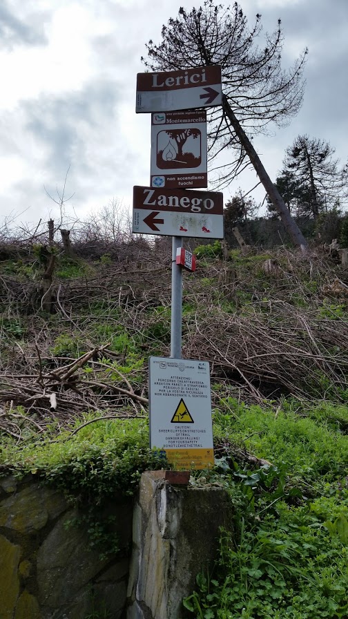
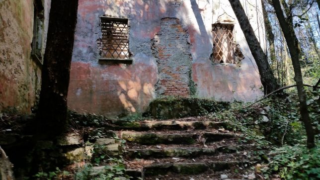
There’s a lot of history in the hills leading up to Monte Rochetta.  On the ascent, you can see old trails and terraces which are long abandoned.  Off of Trail Branzi (one of my favorite, http://www.lericibike.com/2016/05/16/trail-branzi-2-2km/), there are some ruins.  One prominent structure is a hunting lodge built in the 1600s by the Count at the time.  Around the 19th century, frescoes were pained inside which you can still see today. During WW2, this building was actually the home base of a clandestine print press which distributed anti-fascist literature.  The Germans came upon it in 1944 but someone had informed the occupants before they Germans got there to capture them and all that was left was the printing press and the abandoned building.  No one has occupied it since and it stands has pictured today.  Inside there is a plaque which reads (translated into English), “Here at the Rocchetta in the long clandestine silences, simple and courageous men, defying the Nazi-fascist anger, gave new ideas to the press and affirmed in the history the freedom of thought and the right democracy demanded by the resistance. “ [1].

The mountain biking community here is fairly organized and does a good bit of trail maintenance it seems.  There is somewhat of a gentlemen’s agreement whereby you don’t ride the trails for 2 days if it rains.  This is to help keep the trails in good shape.  They also organize beginner rides through the gravel roads and easy trails to help the youth develop their skills and foster an appreciation for the sport. [2]

Many of the trails here are always designated hiking trails which are marked with red and white horizontal lines.  I made the mistake once assuming the markings meant these trails were maintained.  I took a wrong turn once which let me out off a big drop onto the road.  No turning back to go the way I came.  So, I continued on until I found a red and white marked trail.  It was steep with quite a bit of scree — clearly not bikable.  I figured since the trail is marked it can’t be that bad.  Well, it was.  It was at least 100m of scree and I had to carry my bike the entire way.  The work paid off though because I was rewarded with a beautiful view once I reached the top and discovered a local rock climbing area.

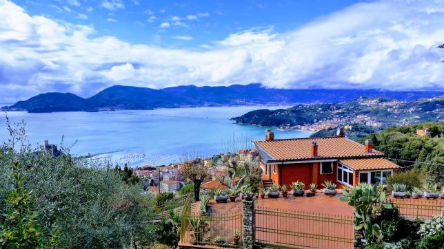
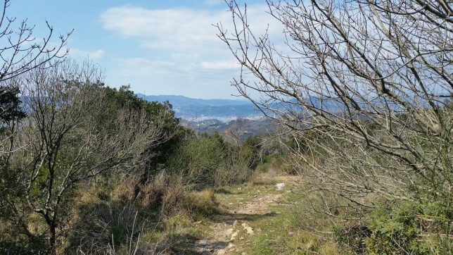
Ok, on to the views!  There are lots of great views along the circuits of trails here.  Vineyards, old camps, panoramas of Lerici, and of course, spectacular views of the Carrara mountains. On trail La Serra, I once ran into a man and his son with a group of what looked like small donkeys.  You never know what you will find on the trails here.

Ciao!

[envira-gallery id=”872″]

References

  1. Clandestine Printing House in Redarca. http://www.tramedilunigiana.it/it/risorsa/monumento/stamperia-clandestina-di-redarca. Fetched 22 April 2018.
  2. Lerici Bike on Facebook. https://www.facebook.com/lericibike/
  3. http://www.lericibike.com/
  4. http://www.lericibike.com/2016/05/16/trail-branzi-2-2km/
  5. https://www.facebook.com/Eurobikes-di-Piero-Arpesella-474552732565146/

Exploring Italy – Take 1

This week has had some really fun adventures.
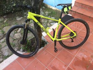
We bought Ryanne and mountain bike and did some riding around Monte Rochetta, Monte Branzi, and Redarca including going down Toranatini (hairpin in Italian). She did really well.

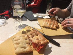
We also took a ride to Tellaoro, the next town over.  This was a pretty easy ride but were able to rack up quite a few miles (km’s that is) and take a small pitstop for some wine and focaccia.

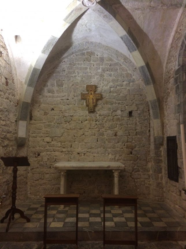
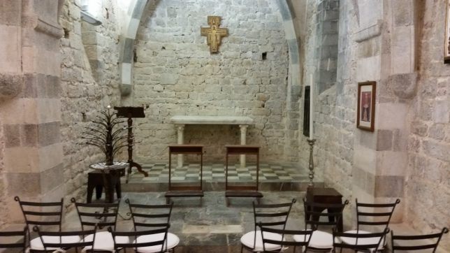
I took Ryanne to see the Castle and the hidden pathways around it.  We were fortunate enough to be able to get into the castle and go all the way to the top — quite the view.  There’s a little sanctuary inside the castle we got a few pics of.

While I was at work one day, our landlady’s took Ryanne out on a hike to Maralunga (another nearby area next to the sea) where they picked wild asparagus. She has also been running mostly daily and exploring the area.  She is quite the adventurer and has herself some nice spots to stop and get coffee, enjoy the sun, and watch the beach-goers.


We have developed an evening ritual of getting gelato at the local place in Piazza Garibaldi. We take a stroll around and catch up on each other’s day while finishing our treat.

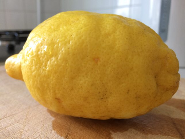
Last night when we stopped at our favorite gelato shop, the place smelled of the strongest, sweetest lemon scent you could imagine. The shop owner hands us a lemon saying to clean, cut, and eat the next morning.  In his kitchen, you could see over a hundred lemons zested to go into his gelato alla crema di limone (which is a favorite of Ryanne).  Showing up daily here has its perks! On the way home, we stopped by the castle to watch some locals play kayak polo.

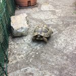
It’s very un-Italian apparently not have a dog.  Most folks we see here have one.  Our home is no different.  In fact, we have 2 dogs and 2 turtles.  The dogs are Rolf and Macchia (which means spot in Italian) and the turtles are named Carletto (Charlie) and Rugetta. Ryanne bought treats for the dogs so they always greet us at the gate when we come home.

A few other random pictures from the week….


Pictures from Italy

Welcome to Italy

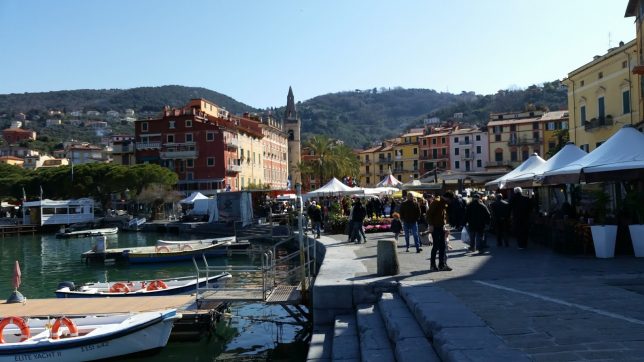
Lerici, Italy

Ryanne arrived here on Sunday (left the USA on Saturday).  Ken and Claire picked her up from the Gerg homestead and took her took the State College airport.  After a long 18 hour trip with three flights and a train ride, we arrived together in our new home in Lerici, Italy! (I took the train to Pisa to pick her up).

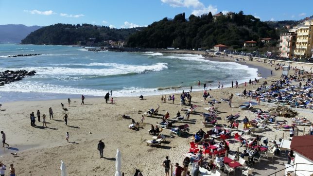
So far Lerici has been very rainy with a few days of beautiful sunshine (and boy is it beautiful when the sun is out).  Apparently, the weather we are seeing is not typical and supposedly should be gone soon.  The temp averages around 55 degrees Fahrenheit going up to 65.

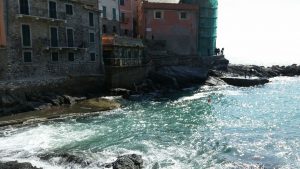
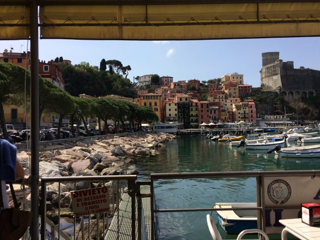
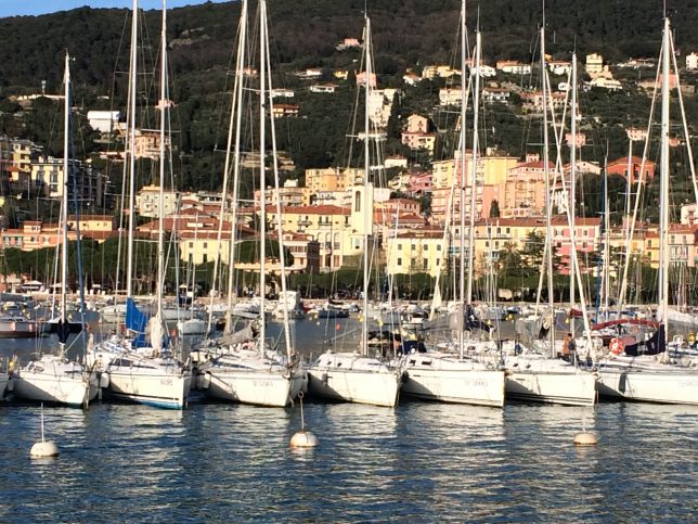
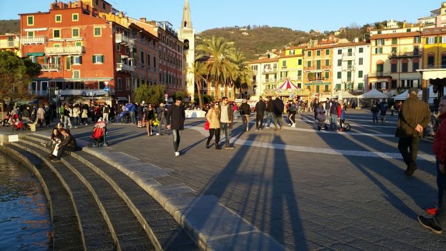
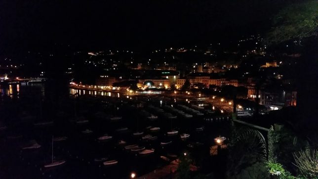
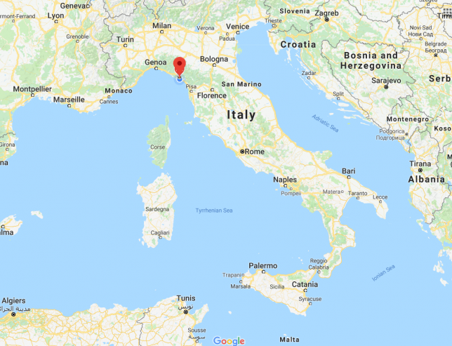
Lerici is on the bay of La Spezia and is bounded by a piazza (Piazza Garibaldi) and Castle Lerici (built around 1100 AD).  The bay is also known as the Golf of the Poets because Mary Shelley (author of Frankenstein) and her husband, Percy, a famous local poet lived in Lerici.  Unfortunately, Percy drowned in the bay and the name was changed as a result in his honor.

Across the Golf of the Poets is the famous Italian Riveria known as the Cinque Terre.  This is on our list of places to visit — stay tuned!

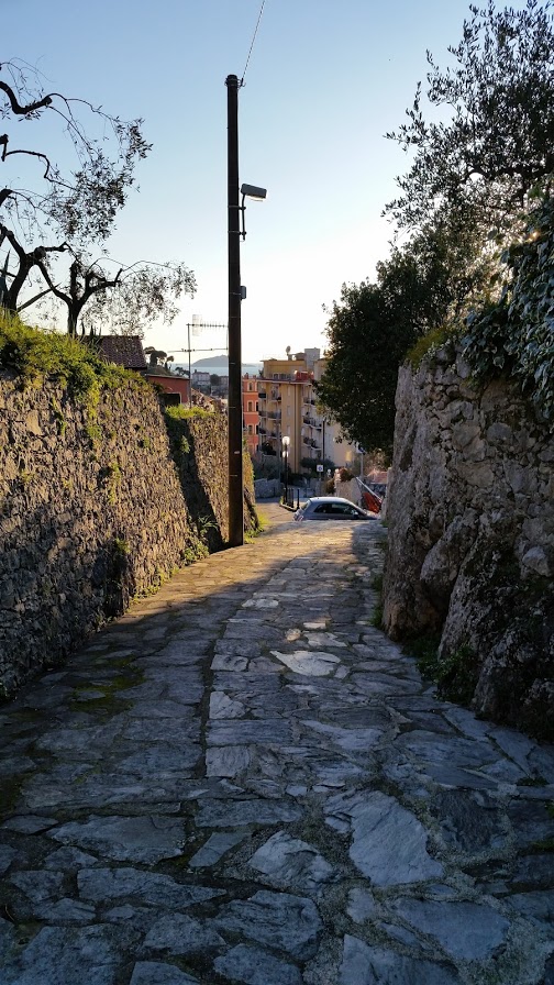
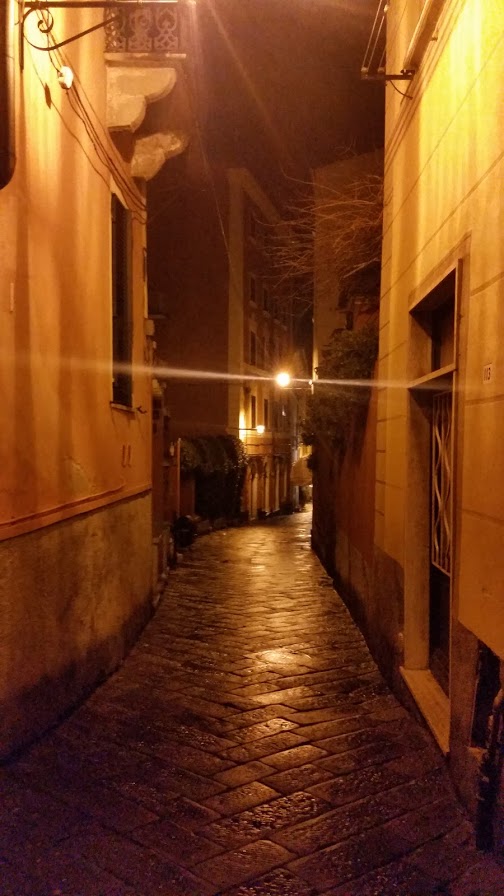
Lerici is essentially built into a hill that rises about 900 feet.  We live about 300 feet up the hillside off a small cobble-stone walkway called XX Settembre.  Its name commemorates a famous Italian date (of which I can’t recall!). The climb up the hillside makes for a perfect post-dinner stroll to work off all the pasta we’ve been eating.  It becomes challenging with a few glasses of wine keeping us on our toes (or on our butts!)


Our bedroom. We have a little “ant problem” hence the creative bed making.

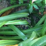
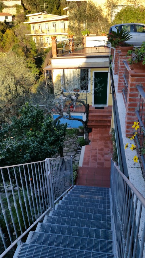
Our “flat” is part of a homestead. We live underneath part of the driveway.  Its hard to explain but it makes sense if you think about the homes being built into a hillside.  Within our homestead, we have citrus and olive trees.  We also have a few pets: 2 turtles (one named Charlie) and 2 dogs (Macchia and Rolf).  We love the dogs and they are Jack Russells.   Makes its really feel like home when you are greeted by man’s best friend.


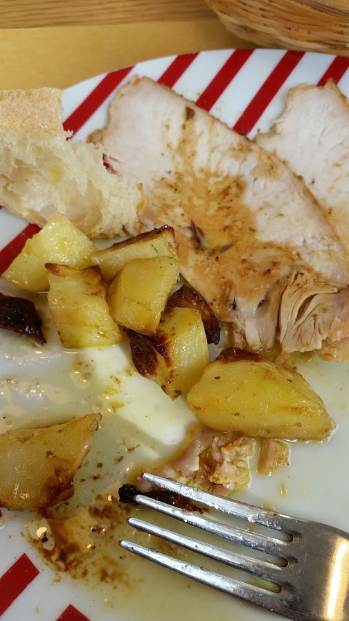
Ryanne made a delicious dinner for us yesterday with local pasta from a place we like called Pasta Fresca and wine from a little shop, Baroni.

Our apartment is small but does the job.  We have a kitchen and breakfast area along with our bedroom and bathroom.  We are lucky enough to have our own washing machine.  No dryer though as most Italians hang their clothes out to dry; we are no different.

Ciao!

~Isaac and Ry


Octopus street graffiti.

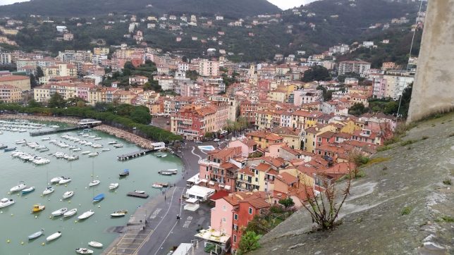
Looking into the bay from up top Castle Lerici.

Lerici, Italy. Our homestead is among the buildings in this picture.

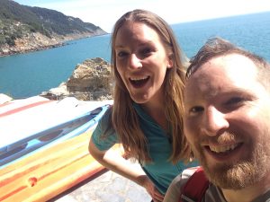
There is a nice walkway along the bay and we stopped to take a selfie.


We had dinner at this interesting restaurant. There is no back room but a cave. We had dinner in it. For dinner, there are no menus; you are told what you will be served. Magically, its what you didn’t know you wanted.


Our friend Macchia.

Changing dropout on the fly (during training time, test time) in keras

I was doing an experiment that involved Monte-Carlo (MC) dropout. I had to change the rate of dropout and have it dropout during test time.

I was able to turn dropout on during test time by making a new function and passing in the learning_phase tensor.

# This code allows dropout to run during test time.
newLayer = K.function([model.layers[0].input, K.learning_phase()], [model.output])
layer_output = newLayer([x, 1])[0] # Dropout on

To change dropout from train time to test time I did the following:

# This code allows you to change the dropout
# Load model from .json
model.load_weights(filenameToModelWeights) # Load weights
model.layers[-2].rate = 0.04  # layer[-2] is my dropout layer, rate is dropout attribute
model = keras.models.clone(model) # If I do not clone, the new rate is never used. Weights are re-init now.
model.load_weights(filenameToModelWeights) # Load weights
model.predict(x)

Reading in Weights from MatConvNet to Keras — Dealing with Keras::Flatten()

Reading in the weights…

 # bastardized from https://aboveintelligent.com/face-recognition-with-keras-and-opencv-2baf2a83b799
 from scipy.io import loadmat
 data = loadmat(weightsFilename,
 matlab_compatible=False,
 struct_as_record=False) 
 
 net = data['net'][0,0]
 net = net.net_params[0,0]
 
 # first conv layer
 tmp = net.layers[1,0][0,0]
 weights = np.zeros((8,8,1,8))
 bias = np.zeros(8)
 for k in range(8):
 weights[:,:,0,k] = np.rot90(tmp.k[0,0][0,k], -2)
 bias[k] = tmp.b[0,k]
 model.layers[1].set_weights([weights, bias])

Keras Flatten() layer gave me some troubles.  In MATLAB, the last level was flattened via…

% concatenate all end layer feature maps into vector
net.fv = [];
for j = 1 : numel(net.layers{n}.a)
 sa = size(net.layers{n}.a{j});
 net.fv = [net.fv; reshape(net.layers{n}.a{j}, sa(1) * sa(2), sa(3))];
end

There is a final Dense layer output 2 classes.  I read the weights in from MATLAB and then mangle them to produce a MATLAB faithful computation.

 # Dense layer
 weights = np.transpose(data['net'][0,0].net_params[0,0].ffW)
 idx = np.arange(300).reshape((5,5,12)).flatten('F')
 idx = np.argsort(idx)
 weights = weights[idx,:]
 bias = data['net'][0,0].net_params[0,0].ffb.flatten()
 
 model.layers[8].set_weights([weights, bias])

Essentially, I mimic the forward mangling process.  MATLAB is column major.  So, I create a vector of 300 elements from 0 to 299 (my last conv layer output is 5x5x12). I flatten this vector using FORTRAN style flattening.  Now, I must get the reverse mapping which is accomplished via and argsort.  Finally, I reorder the MATLAB weight vector so that when keras reorders via flatten(), its in the same ordering as the MATLAB MatConvNet computation.

net.o = sigm(net.ffW * net.fv + repmat(net.ffb, 1, size(net.fv, 2)));

10 Acre Pond, Scotia

How Our Life Has Changed in Ten Years

In 2007,

  • The first iPhone was release.
  • GPU computing was coming into mainstream, CUDA 1.0 released.
  • The Samsung Galaxy phone didn’t exist yet.
  • The first year you longer need an invitation to get a gmail account.
  • In February 2007, the Nintendo wii outsells the XBOX and Ps4 (https://www.technologyreview.com/s/408183/hack-the-nintendo-wii/)
  • The first Amazon Kindle is released (https://en.wikipedia.org/wiki/Amazon_Kindle)
  • There is no 4G network for cell phones.
  • Deep Learning doesn’t exist.
  • There is no imagenet benchmark for object recognition.
  • In the Top 500 supercomputer list, entry to the top 50 requires 16 Teraflops. NVIDIA GPUs you purchase at Best Buy can do 10 Teraflops.(ttps://www.top500.org/lists/2007/06/highlights/, http://www.bestbuy.com/site/evga-geforce-gtx-titan-x-12gb-gddr5-pci-express-graphics-card-black/5550016.p?skuId=5550016)
  • The NIH launches the Human  Microbiome Project (https://www.nih.gov/news-events/news-releases/nih-launches-human-microbiome-project)
  • Wikipedia had 1.5 million English articles.  Today its around 5 million. (https://blog.wikimedia.org/2015/11/01/english-wikipedia-surpasses-five-million-articles/)

Installing Tensorflow in Windows 7 x64 for Python 3.5

Here are my instructions to install Tensorflow (tf) in Windows 7 x64 for Python 3.5.  I have verified these instructions work to get tf working with Keras.  e sure to update your keras.json file to use the tf backend if you already use theano.  You do not need to purchase visual studio to get this to work.

I. Prerequisites

  1. Install Cuda 8.0.  Note, you must use the release version of 8.0 and NOT the release candidate.
  2. Install python35 to c:\python35 (no need for anaconda)
  3. Download cudnn (record path)
  4. Download swig (record path)
  5. Install visual studio 2015 community edition with C++.  Had to manually install c++ in visual studio 2015 community edition. went into control panel, programs and features, and did a modify
  6. Install git for windows

II. Getting the tf repository

  1. git clone https://github.com/tensorflow/tensorflow.git
  2. cd tensorflow\tensorflow\contrib\cmake
  3. mkdir build
  4. cd build

III. Begin the tf install

  1.  “C:\Program Files (x86)\Microsoft Visual Studio 14.0\VC\bin\amd64\vcvarsall.bat” (make sure you are using the amd64 version)
  2. cmake .. -A x64 -DCMAKE_BUILD_TYPE=Release -DSWIG_EXECUTABLE=d:/swigwin-3.0.10/swig.exe -DPYTHON_EXECUTABLE=c:/python35/python.exe -DPYTHON_LIBRARIES=C:/Python35/libspython35.lib -Dtensorflow_ENABLE_GPU=ON -DCUDNN_HOME=D:/ASASINATR/cudnn -Dtensorflow_ENABLE_GPU=ON
  3. MSBuild /p:Configuration=Release tf_tutorials_example_trainer.vcxproj
  4. Release\tf_tutorials_example_trainer.exe (this should work if everything built correctly)

IV. Make the python wheel

  1. pip install travis pip setuptools wheel
  2. MSBuild /p:Configuration=Release tf_python_build_pip_package.vcxproj
  3. pip install D:\tensorflow\tensorflow\tensorflow\contrib\cmake\build\tf_python\dist\tensorflow-0.11.0rc2_cmake_experimental-py3-none-any.whl

If everything was successful you should be able to modify your keras.json file, load keras in python, and begin using tf.


Thanks to Derek Murray of Google for the help creating this.

Installing Theano in Windows 7 with Python 3.4

I recently upgraded my machine learning toolchain to keras and thought it would be a good time to revisit the ongoing theano + Python 3.4 + Windows 7 saga.  I found a simple set of instructions here which I tweaked a bit to get to work with my setup.  Here are the full instructions:

  1. Install python 64bit
  2. Install precompiled whl from http://www.lfd.uci.edu/~gohlke/pythonlibs
    1. Numpy+MKL library
    2. scipy
  3. Get GCC from http://tdm-gcc.tdragon.net/ (I usually have issues with GCC in Windows, however, this distribution works great out of the box believe it or not)
  4. Install theano via pip and http://www.lfd.uci.edu/~gohlke/pythonlibs
  5. At this point, when I tried to import theano into python 3.4, I would get linking errors.  I then installed libpython from http://www.lfd.uci.edu/~gohlke/pythonlibs and that resolved the issue.
  6. At the python shell, type import theano, it should work
  7. Configure your .theanorc.txt and you should be good to go.

uBiota, A New Startup Examining Your Microbiome

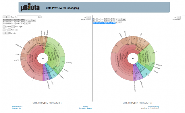
I was fortunate enough to have 3 samples of what I will call “gut” bacteria (you fill in the blanks) examined by a new startup, uBiota.  I have to say, I am impressed with their visualization.  Its very interactive and easy to use.  I really like the search function.

ubiota1


A picture is worth a thousand words, but click here and you can test drive it for yourself.

The three samples were taken on:

  1. 10-9-2015
  2. 10-6-2015 – Also analyzed by Genova Diagnostics.
  3. 10-1-2015

Apologies for not taking the samples in time order.  The second sample I also had analyzed by Genova Diagnostics for comparison. I will post results at a later date.

Full disclosure – I was given 3 sampling kits for free from uBiota.

CX 20 Cheat Sheet

SWB   SWA   Description
 0     1    Stable mode - position hold mode.
 0     2    Return to home mode
 1     1    Flight direction lock
 1     2    Altitude mode, drive at a fixed altitude (may run into hills).  Don't have to use the throttle (left paddle up-down)

Flight stability Calibration Left control pressed down left - red and green lights will blink - fly off ground for 20 seconds - lock and unlock on ground to save settings. Compass Calibration As soon as you power on the drone, turn the tx on and push the right paddle to the bottom right corner. The lights will eventually flicker yellow and green. Pick up the drone by the base keeping it level and spin yourself around 3-5 times. Now hold the drone so that front (opposite side of the battery pack access panel) is facing the floor and spin yourself again holding the drone 3-5 times. Now, place the drone on a level surface and disconnect the power. See this youtube for an example: https://www.youtube.com/watch?v=uz4_8RYXeD0 Switch controller off - drone will land auto land where tx is

Left control pressed down left - lock motors - red light blinks 
Left control pressed down right - lock motors - red light solid

GPS lock -    green light solid
No GPS lock - green light blinking

Bottom lights blinking and drone blinking - drone battery low
Beeping on the controller means the throttle (left paddle) is in the middle.

Aux knobs are for controlling a gimbal.

images2gif.py for Python 3

I took the images2gif.py class (https://bitbucket.org/bench/images2gif.py) and modified it to work with Python 3.  Most of the work involved moving from str type to bytes.

Code is on github (https://github.com/isaacgerg/images2gif).


Plants Around the Yard

Record of the plants around my yard because I am a science nerd.

(more…)

PicnicHealth.com

This is my first entry promoting something. I dislike when others do it but I am making an exception because this service has significantly helped me. The company is called PicnicHealth and their website is http://www.picnichealth.com.

Since returning from Italy last year, I have been plagued with chronic stomach dysfunction. I have seen several doctors including a specialist at John Hopkins Medical Center. I have had to go through all the pain of collating my notes, labs, imaging studies, etc.  to send to doctors and analyze myself. Its been a pain until I found this tool through an article about PicnicHeath and uBiome collaborating. I follow uBiome semi-regularly as a personal interest.

They have a legitimate DICOM viewer so all my medical imaging shows up great, including the adjustments for brightness, contrast, and movie playback controls.

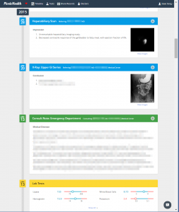
Anyways, here’s a quick sample of what my health timeline looks like.

picnichealth_example

Installing Theano in Windows 7 64-bit

My instructions for installing Theano 0.6 with

  • Windows 7-64 bit
  • Anaconda 2.1.0 (Python 2.7).  This tutorial only works with 2.1.0.  I tested it with 2.2.0 and it did not work.  I have no plans to fix this issue.
  • CUDA 7.0

Steps

  1. Download Anaconda 2.1.0 from here.
  2. Install pip via command line using “pip install https://pypi.python.org/packages/source/T/Theano/Theano-0.6.0.zip#md5=0a2211b250c358809014adb945dd0ba7
  3. Create a .theanorc.txt file in your user area (C:\Users\username\.theanorc.txt) with the specified text listed below.
  4. Open Anaconda
  5. Import and test/build theano by typeing import theano and then theano.test()
  6. Sit back and relax while everything builds.

.theanorc.txt file contents (you must create at %USERDIR%/.theanorc.txt, for me this is c:\users\username\.theanorc.txt)

[global]
openmp=False
device = gpu0
floatX = float32

[blas] ldflags=

Notes

If you get an error about “CVM,” you must delete the cache files that are in C:\Users\MyUsername\AppData\Local\Theano. Once you delete everything, start python again and continue from there.

If you have path issues when trying to import theano, try using the Visual Studio 64-bit command prompt if you have it.  It sets a bunch of paths for you and “just works” for me.  For reference, the path I use is:

PATH=C:\Program Files (x86)\Microsoft Visual Studio 10.0\VC\BIN\amd64;C:\Windows\Microsoft.NET\Framework64\v4.0.30319;C:\Windows\Microsoft.NET\Framework64\v3.5;C:\Program Files (x86)\Microsoft Visual
Studio 10.0\VC\VCPackages;C:\Program Files (x86)\Microsoft Visual Studio 10.0\Common7\IDE;C:\Program Files (x86)\Microsoft Visual Studio 10.0\Common7\Tools;C:\Program Files (x86)\HTML Help Workshop;C:
\Program Files (x86)\Microsoft SDKs\Windows\v7.0A\bin\NETFX 4.0 Tools\x64;C:\Program Files (x86)\Microsoft SDKs\Windows\v7.0A\bin\x64;C:\Program Files (x86)\Microsoft SDKs\Windows\v7.0A\bin;C:\Program
 Files\NVIDIA GPU Computing Toolkit\CUDA\v7.0\bin;C:\Program Files\NVIDIA GPU Computing Toolkit\CUDA\v7.0\libnvvp;C:\Python34\Lib\site-packages\PyQt5;C:\Program Files (x86)\NVIDIA Corporation\PhysX\Co
mmon;C:\Program Files\NVIDIA GPU Computing Toolkit\CUDA\v6.5\bin;C:\Program Files\NVIDIA GPU Computing Toolkit\CUDA\v6.5\libnvvp;C:\Program Files (x86)\Intel\iCLS Client\;C:\Program Files\Intel\iCLS C
lient\;C:\Windows\system32;C:\Windows;C:\Windows\System32\Wbem;C:\Windows\System32\WindowsPowerShell\v1.0\;C:\Program Files\Intel\Intel(R) Management Engine Components\DAL;C:\Program Files\Intel\Intel
(R) Management Engine Components\IPT;C:\Program Files (x86)\Intel\Intel(R) Management Engine Components\DAL;C:\Program Files (x86)\Intel\Intel(R) Management Engine Components\IPT;C:\Program Files\MATL
AB\R2014a\bin;C:\Program Files\TortoiseHg\;C:\Program Files (x86)\Microsoft SQL Server\100\Tools\Binn\;C:\Program Files\Microsoft SQL Server\100\Tools\Binn\;C:\Program Files\Microsoft SQL Server\100\D
TS\Binn\;C:\Users\username\AppData\Local\Continuum\Anaconda;C:\Users\username\AppData\Local\Continuum\Anaconda\Scripts

Update June 11, 2015
Added link to Ananconda download

Block Fun

Compute the number of blocks, k, given a window size, w, overlap size, p, and number of points, N.

[latex]k =\lfloor\frac{N-w}{w-p}\rfloor + 1[/latex]

Getting QGraphicsView with a pixmap to Zoom and Scroll Like the Window’s Photo Viewer

This took me forever to figure out.  I noticed lots of people online had the same question but few got it working properly and some had to do a hack.  Here is the clean way to do this.  The trick is in setTransformationAnchor() and setDragMode()

My setup code in my QDailogs __init__ function:

imageFilename = QFileDialog.getOpenFileName(self,'select image')
self._pixMap = QPixmap.fromImage(QImage(imageFilename)) 
self._graphicsScene = QGraphicsScene(self)
self._graphicsScene.addPixmap(self._pixMap)
self._view = MyGraphicsView()
self._view.setScene(self._graphicsScene)

# Create a vertical layout.
self._layout = QVBoxLayout()
self._layout.setMargin(0)
self._layout.setSpacing(0)

# Add label widget
self._layout.addWidget(self._view)
# set widget to layout
self.setLayout(self._layout)


Here is my implementation of the MyGraphicsView class.  Derived from QGraphicsView

class MyGraphicsView(QGraphicsView):
    def __init__(self):
        QGraphicsView.__init__(self)
        self.setRenderHints(QPainter.Antialiasing|QPainter.SmoothPixmapTransform)
        self.setTransformationAnchor(QGraphicsView.AnchorUnderMouse)
        self.setDragMode(QGraphicsView.ScrollHandDrag)
    def wheelEvent(self,event):        
        adj = (event.delta()/120) * 0.1
        self.scale(1+adj,1+adj)

Glider Ride

Went out to Ridge Soaring Gliderport for a flight last Friday.  Doris Grove was my awesome pilot. Check it…


Morocco Trip – 2011

Would like to write something about this eventually.  Here are some pics.

This was a last minute trip literally — booked my plane tickets and a week later was in Casablanca.  Would like to write something about budget travel, traveling like you live there, and how you don’t need to have a plan to travel but still be safe.

Simple UHD Transceiver Class

I wrote a simple transceiver class for the USRP1 (GNURadio) using the new UHD interface.

The class allows you to send and receive data.  What you fill in for the data is up to you.  Currently, the class performs simple energy detection (sends a 100 sample burst with constant envelope) and works when you hook the RX up to the TX on the Basic RX/TX boards (make sure you have proper attenuation as to not break the daughterboards).  But, with some simple modification, you can have it do more sophisticated processing.

The class creates two queues and three threads.

One queue is the TX queue and the other the RX queue. The TX queue is a vector of pointers to complex float vectors (variable length) and are waveforms to be transmitted. The RX queue is a vector of pointers to complex float vectors (const size) and are the data blocks received from the radio.

The three threads are the TX thread, the RX thread, and the processing thread.

The TX thread wakes up every 100ms and looks at the TX queue and sends any waveforms that are present.  The RX thread runs continuously and receives datablocks from the radio. The processing thread checks the RX queue and processes any blocks that are present on it.  Having an RX queue, RX thread, and processing thread allows the software to continually receive data without dropping packets and leaves the choice up to the software as to which packets to process.  For example, if the processing thread runs slower than the samples coming in (slower than real time), it may choose to intelligently process the remaining blocks instead of dropping data on the floor.  This would allow the processing thread to “catch up.”

The TX thread can be modified as to send the waveforms out immediately instead of on a queue for servicing.

I hope all this makes sense.

The code can be downloaded here.  I used this to compile:

g++ main.cpp SimpleTransceiver.cpp -lboost_thread -luhd -I/opt/uhd/include -L/opt/uhd/lib

Bugs, questions, comments welcomed.

Enjoy!

Getting Boost to Compile Correctly with Visual Studio 10 & CUDA on a 64-bit Machine

Sexy title, I know!

Anyways, I’m developing using Visual Studio 10 (not my choice).  I have a project which involves the use of CUDA and Boost. The newest version of CUDA (at the time of this writing) won’t work out of the box with the  vs100 compiler that comes with Visual Studio 10.  CUDA can use nothing newer than the vs90 compiler.  So, I  install visual studio 9 and 10 and select v90 as my compiler for my Visual Studio 10 project.

Yesterday, I needed the Boost C++ libraries and began to install them.

The Boost installation is pretty good.  Its fairly automated which is nice.  You essentially call bootstrap and then bjam; they take care of all the configuring and building of the .libs.  However,  Boost’s scripts see that I have Visual Studio 10 installed and compile everything with the vs100 compiler.  This breaks my project in  Visual   Studio (I get all linking errors related to Boost) as I’m in  Visual Studio 10, but using the v90 compiler because of CUDA.

So, I figured out how to override Boost’s configuration to compile with the vn90 compiler instead of the vc100 compiler.  Here is how I fixed the problem.

 cd to BOOST_ROOT
 boostrap
 "C:\Program Files (x86)\Microsoft Visual Studio 9.0\VC\bin\vcvars64.bat"    // This invokes the vc90 environment variable set.
 bjam --toolset=msvc-9.0 --build-type=complete architecture=x86 address-model=64  // Makes Boost!

If you don’t run the 3rd line (vsvars64.bat), you will see tons of “cl” errors when running  bjam.  Essentially, Boost tries to call the vc90 compiler (cl.exe), but because the environment is hosed, it cant find it and bombs.

Useful Bits of MATLAB

Generating a unique ID (UID):

uid = floor((now – floor(now))*1e8);

Pictures from Estonia

I have posted my pictures from my Estonia 2010 missions trip.  They are here.

Here are a few of my favorites…

Estonia Trip Mentioned in State College Town & Gown

The missions trip I have previously taken to (and will take again this year very soon) Estonia was mentioned in State College, PA’s Town & Gown magazine.  The article is here.

Seg-2 Reader for MATLAB

So I have been looking for a seg-2 reader for MATLAB for some time now.  For those of you who don’t know, seg-2 is a file format for storing seismic data.  Anyways, I’ve googled “seg-2 reader  MATLAB” for sometime and came up with some shareware software and some broken links pointing to MATLAB code.

Today, I have found some MATLAB code here.  For posterity, I will post the code here as I do not know the volatility of the site hosting the code.

USRP / Simulink Interface

I had been looking for some time for an interface for the USRP/GNU Radio to MATLAB Simulink. Well, I went looking through the MATLAB forums today and saw that someone responded to my post.  I checked the GNU Radio forums to make sure this information was seen to the users of that listserv.  I found where it was announced on there though the link didn’t work.  However, I did some searching and found the interface here.

Fixing My 2004 Saturn Ion Winshield Wiper Linkage

About a week ago, my driver-side windshield wiper starting behaving strangely.  The wiper would move too far to the left and not always go back to its wiper-home when turned off.  It also seemed to move in a delayed fashion when in comparison to the passenger-side wiper.  When passengers asked about it, I compared it to a lazy eye.

In the beginning, the wiper would clean the windshield for the most part, but it soon got worse.  I came back to my childhood home for Christmas to visit my parents.  As most parents would, my dad noticed the bad wiper and asked me why I didn’t fix it.  As most single twenty-somethings would, I said I’d get around to it; after all, I could still see good enough to drive.  In the meantime, my dad googled the problem and found several people who had the same problem.  As it turns out, the windshield wiper linkage broke.  Then can happen when you pull back the wipers off the windshield and reapply them without being careful.  I usually pulled back my wipers when it snows to prevent them from sticking to the windshield and then just pushed them back, in which they would smack the windshield.  I had good intentions, but poor execution; lesson learned.

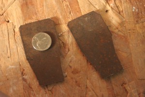
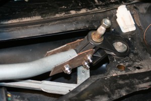
My dad and I began to take apart the windshield wiper apart.  We confirmed the linkage was broken.  We then used the instructions from here to fix the problem.  We fixed the problem by repairing the broken part with two metal pieces and some bolts.  The repair worked and all is well!

You can click on the pictures below for a larger view.

Broken linkage

Removed wiper motor from car

Brackets to repair the break

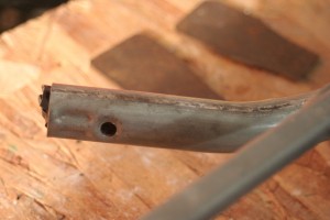
First hole drilled in the linkage for the repair

Fixed linkaged reinstalled in the car

Debricking a Linksys WRT54GS v5.0 Router

I’ve been looking at the logs for this site and have noticed that many people come here looking for the article on debricking a Linksys WRT54GS router (March 31st, 2007), an article on my old blog.  Well, I had lost the article when I switched web content solutions but just found it in the Internet Archive Wayback Machine.  I have reposted the article below.

I have a Linksys WRT54GS v5.0 router that I purchased from ebay. I bought it because I had heard that installing DD-WRT firmware on these router versions was difficult and many people manage to brick them. I wanted to see for myself.

I began to install the 3 firmwares required to get DD-WRT working (pre, vxWorks killer, and finally DD-WRT mini). I managed to brick the router after trying to install the 3rd and final firmware. The router would not respond to anything: ping, Linksys TFTP, and manual network configuring. I looked all over the internet to find way to debrick this router and find two method:

  1. JTAG cable
  2. Pin shorting

I didnt have a JTAG cable nor wanted to buy one. So, I tried the pin shorting as a last resort. So I used the tutorial I found and shorted pin 4 and 5 with a jewelry screwdriver and viola, the router started to respond. I then tried to install the firmware again but ended up bricking the router several more times. So, I switched to another firmware installation HOWTO. It seemed to let me install the firmware via TFTP but not the web interface because it would not come up. So, I just followed all the usual instructions but instead installed the firmwares using TFTP. Everything worked fine up until the final firmware. The router didnt brick this time, but the webpage would not come up. I then read in a forum somewhere that you have to wait up to 10 minutes after installing the last firmware before the webpages will come up. I waited and it worked.

I am now using my bricked WRT54GS router with DD-WRT micro on it!

The link to the tutorial to upgrade to DD-WRT that worked:

http://www.bitsum.com/openwiking/owbase/ow.asp?WRT54G5%5FCFE#h10

The link to the tutorial to short pins 4 and 5. It says its for the G but I got it work with the GS; just be sure to short pins 4 and 5 (USE AT YOUR OWN RISK!):

http://voidmain.is-a-geek.net/redhat/wrt54g_revival.html

RIT Hyperspectral Target Detection Blind Test Forum

I have emailed John Kerekes of RIT about getting a forum set up for this contest.  He thinks it is a good idea, so I went ahead today and set on up.  The forum is http://n3.nabble.com/RIT-Hyperspectral-Target-Detection-Blind-Test-Forum-f48632.html .

Enjoy.

RIT Hyperpsectral Target Recognition Contest

RIT is currently hosting a hyperspectral target recognition contest.  They group provides a training set and a test set.  You run your algorithm on the test set and then submit your results via web browser.  The website scores you and determines your rank.

I won’t go into much more detail of the contest.  Go to the website, get an account, and check it out for yourself.  I am interested though in getting a forum or listserv together so folks working on the project can collaborate (there is no prize money involved).  I have solicited RITto see if they are willing to put together such a forum or listserv.  I will keep everyone posted on what I find.  If nothing happens, I’ll start one and host it here.

In the meantime, I’m curious to know who is all competing in this contest.

Popular Hyperspectral Target Detection Kernels

I’ve been implementing several hyperspectral target detection algorithms for the Matlab Hyperspectral Toolbox.  I am going to use this post to summarize my research and implementations.  It will take me a few days to  get all my thoughts together, so this note will be a “living post” over the next week or so.  Please email me if you find any errors or something is not explained clearly.  I can be contacted at first.last-At-gergltd.com.  Thanks, Isaac Gerg

Notation

[latex]p[/latex] – Number of bands.  E.g. for AVIRIS p = 224.

[latex]N[/latex] – Number of pixels.

[latex]q[/latex] – Number of materials in the scene.

[latex]\mathbf{M}[/latex] – Matrix of hyperspectral imagery (HSI) data. Size is (p x N).

[latex]\mathbf{x}[/latex] – Observation vector, a pixel.  Size is (p x 1).

[latex]\mathbf{\mu}[/latex] – Data mean.  Size is (p x 1).

[latex]\mathbf{t}[/latex] – Target of interest.  Size is (p x 1).

[latex]\mathbf{\Gamma}[/latex] – Covariance matrix of M.  Size is (p x p).  [latex]\mathbf{\Gamma} = \frac{(\mathbf{M}-\mathbf{\mu}\mathbf{1}^T)(\mathbf{M}-\mathbf{\mu}\mathbf{1}^T)^T}{N}[/latex]

[latex]\mathbf{R}[/latex] – Correlation matrix of M. Size is (p x p). [latex]\mathbf{R} = \frac{\mathbf{M}\mathbf{M}^T}{N}[/latex]

[latex]\mathbf{U}[/latex] – Matrix of background endmembers. Size is (p x q).

[latex]\mathbf{P}_{U}^{\perp}[/latex] – Orthogonal projection of [latex]\mathbf{U}[/latex].  [latex]\mathbf{P}_{U}^{\perp} = \mathbf{I} – \mathbf{U}\mathbf{U}^{\dagger}[/latex]

Kernels

Assume the mean has been removed from the data unless otherwise noted. Assume these kernels work on radiance or reflectance data unless otherwise noted.

RX Detector

[latex]D_{RX Detector}(\mathbf{x}) = \mathbf{x}^T\mathbf{\Gamma}^{-1}\mathbf{x}[/latex]

Matched Filter (MF)

[latex]D_{Matched Filter}(\mathbf{x}) = \frac{\mathbf{x}^T\mathbf{\Gamma}^{-1}\mathbf{t}}{\mathbf{t}^T\mathbf{\Gamma}^{-1}\mathbf{t} }[/latex]

Adaptive Coherent/Cosine Estimator (ACE)

[latex]D_{ACE}(\mathbf{x}) = \frac{(\mathbf{t}^T\mathbf{\Gamma}^{-1}\mathbf{x})^2}{(\mathbf{t}^T\mathbf{\Gamma}^{-1}\mathbf{t})(\mathbf{x}^T\mathbf{\Gamma}^{-1}\mathbf{x}) }[/latex]

Constrained Energy Minimization (CEM)

[latex]\mathbf{x}[/latex] and [latex]\mathbf{t}[/latex] are not centered for this algorithm.  I.e. Do not remove the mean of the data when computing this kernel.

[latex]D_{CEM}(\mathbf{x}) = \frac{\mathbf{t}^T\mathbf{R}^{-1}\mathbf{x}}{\mathbf{t}^T\mathbf{R}^{-1}\mathbf{t} }[/latex]

Generalized Likelihood Ratio Test (GLRT)

[latex]D_{GLRT}(\mathbf{x}) = \frac{(\mathbf{t}^T\mathbf{\Gamma}^{-1}\mathbf{x})^2}{(\mathbf{t}^T\mathbf{\Gamma}^{-1}\mathbf{t}) (1 + \mathbf{x}^T\mathbf{\Gamma}^{-1}\mathbf{x})}[/latex]

Orthogonal Subspace Projection (OSP)

[latex]D_{OSP}(\mathbf{x}) =  \mathbf{t}^T \mathbf{P}_{U}^{\perp} \mathbf{x} [/latex]

Adaptive Matched Subspace Detector (AMDS)

B is a matrix of background signatures.  Size is (p x q).  Z is a matrix of background and target signatures.  Size is (p x (q + # targets)).

[latex]D_{AMDS}(\mathbf{x})=\frac{\mathbf{x}^{T}(\mathbf{P}_{B}^{\perp} – \mathbf{P}_{Z}^{\perp})\mathbf{x}}{\mathbf{x}^{T}\mathbf{P}_{Z}^{\perp}\mathbf{x}}[/latex]

More to come…..

Matlab and the AMD Athlon XP 3200+

So I just purchased a person copy of Matlab.  I start to run my hyperspectral toolbox upon it only to be greeted with Matlab segfaulting.  I traced back the error to the inv() and eig() functions.  For a little test, I constructed a one line program that invokes the crash:  clear; inv(eye(2));

Now, I begin to dig and dig to find the reason for the problem.  I search Mathwork’s website, I file a bug report, and I search Google.  I finally find an answer to my question here.  To make a long story short, Matlab R2009a does not support processors that don’t support SSE2 instructions.  This is ridiculous!  It’s one thing to support backwards compatibility for software, but not for x86 compliant hardware?

I just bought a netbook which runs an Intel Atom and supports the SSE2 instructions set.  I attempted to install Matlab on that machine, since it was my server that Matlab won’t current run on, only to run into licensing issues since the licence is tied to a hardware ID.  This story is still unfolding — another story for another time.

Matlab Hyperspectral Toolbox Released!

I just released my Matlab Hyperspectral Toolbox.  Its available for download at:

http://sourceforge.net/projects/matlabhyperspec/files/

There are separate downloads for the code and the sample data files.  Im still getting the hang of how to handle sourceforge.net, but will have a webpage (wiki) up soon.

The current release features a function called hyperDemo which demonstrates two fully unsupervised exploitation chains, one utilizing ATGP and one utilizing ICA.

I am hoping in the next week to publish methods for doing ACE  as well as a few others.
Enjoy!

PS:  Project website now working and is located at: http://matlabhyperspec.sourceforge.net/

Google Chrome & Firefox SSL and CSS Display Issues

Recently, I resurrected an old computer given to me by a friend. I installed a legal version of XP on it and began to install my usual software. I installed Google Chrome and Firefox. One day, I noticed Google Chrome was processing flickr.com’s login strangely: Chrome was given me a warning about SSL certificates and not rendering the CSS. I was really confused. After doing some searching, I figured out the issue: I had not properly read the SSL warning and realized by computer’s clock was set in the year 2000.

SSL Weirdness

SSL Weirdness

CSS Processing Weirdness

CSS Processing Weirdness

Did you catch the SSL error carefully?   It says that “the server’s security certificate is not yet valid.”  I didn’t catch it at first.  I just assumed it was warning me about an incorrectly signed certificate like Chrome sometimes gives me.

To fix the problem, I simply set my clock to the correct time and then the SSL warning went away and the flickr login page began to render correctly.

I experienced this problem with Firefox also and the above method fixed my issues their also.

Matlab Hyperspectral Toolbox

I developed a Matlab hyperspectral toolbox as part of my Master’s thesis during 2006-2008.  I am currently in the midst of updating the documentation and cleaning the code.  I will release this code shortly on sourceforge and begin continued work on the toolbox.  Currently, the toolbox will have algorithms to estimate the number of materials in an HSI scene, compute endmembers, and compute material abundance maps (MAMs) using different constrained least square techniques.  I will be providing a demo with the toolbox which demonstrates usage of the functions to help everyone understand how to use the toolbox.
I plan on adding several HSI algorithms as well including:

  • ACE
  • GLRT
  • OSP
  • Sof the algorithms Josh Broadwater of JPL has come up with that are based on constrained least squares methods.
  • RX detector
  • New super-resolution methods based on material abundance map information
  • MNF
  • Destreaking algorithm (for processing Hyperion data)

If you are interested in getting involved with the project, please email me at first.last -At- gergltd.com.  If you are a current Penn State Schreyer Honors College student looking for a thesis topic, I have lots of possible projects for you to work on and money to fund you through Penn State.

Useful Canon Rebel XT Resources

I am always doing research about my Canon Rebel XT 8MP (aka 350D) camera. Below are some resources I have found useful.

  1. Parameter Settings – Examines the settings of contrast and sharpness.  I strive to do as little as post-processing as possible as it takes time.  So, I try to work with the camera to have it do as much work as possible.
  2. Google Book of Rebel XT – I bought this book.  Here is the google book version of it.
  3. How one person configures their parameters (i.e. contrast, saturation, etc)

Commonly Used Linux Commands

Some Linux commands I find useful.

tar -xvjpf file.tar.bz2
bunzip2 file.bz2

tar -xzf file.tgz
find . -name file.txt -print

Estonia Trip

I just returned back from my trip to Estonia.  I have posted many pictures including some HDR’s I took.  The pictures are available here: http://gergltd.com/zenphoto/2009%20-%20Estonia/

Tips on Using Qtpfsgui to Produce HDR Images

I currently use Qtpfsgui 1.9.3 to assemble my photographs into high dynamic range (HDR) images.  In this tool, I am currently using the Mantiuk algorithm.  I find Mantiuk has only a few knobs to turn and yields great results.

I’ve developed a nice workflow in using the Mantiuk algorithm.  I generally leave the contrast settings alone, crank up the saturation to around 1.8, and then vary the detail between 1.0 and 3.0 depending on the picture.

Recently, I’ve found a good use of the contrast adjustment of Mantiuk and want to share my findings.  The image below shows my initial adjustments using Mantiuk.

Initial adjustments using Mantiuk

Initial adjustments using Mantiuk

Notice how the light is stratified vertically below the clouds.  I found that turning up the contrast help alleviate this effect.  In the following image, I turned it up a good amount to highlight the difference.

With contrast setting increased

With contrast setting increased

Fixing Counterize II When Stats Not Updating

I use the wordpress plugin Counterize II to track who visits my websites.  I recently noticed the plugin did not report any information for one of my sites.  At first I thought it was a database issue, but upon looking into it, this was not the case.

I tried all sorts of methods to fix it: I deactivated and reactived the plugin, uninstalled and reinstalled the plugin, and messed around with the database tables.  None of these methods worked.

As a last resort, I thought it could be related to the theme I was using since I had made some changes to it.  I double checked all the changes I made and they all seemed benign.  So, I began to look through the Counterize II code to see what function actually gets called to record the site hits and how it gets called.

It turns out, that Counterize II gets called through a wordpress API hook.  Looking further into the problem, I realized that my theme never calls the function that is to invoke the hooks, specifically, the wp_head() function.

After some more searching, I found this website which helped me fix my problem.  For Counterize II to function, you have to have

<?php wp_head(); ?>

somewhere inside your <head> HTML section.  I added that line of code and Counterize II now works!

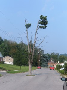
Haunted Tree in Huntingdon, PA

Picture of the imfamous tree in the middle of the road

Picture of the infamous tree in the middle of the road

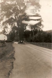
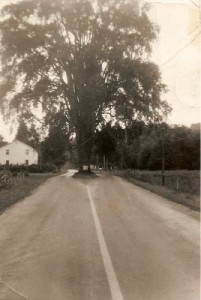
UPDATE: December 26, 2013 – Carl Naples sent me pictures of the tree from 1957-58.  Added to end of post.

Back in 2004, I did some hiking at the Thousand Steps trail in Mount Union, PA.  I discovered the trail while looking online for good hiking trails nearby State College.  I also found during this search a story about a tree in the middle of the road in Huntingdon, PA, a town on the way to Mount Union.  Could this story be true?

There is a tree, literally, in the middle of a paved road on a side street right off of Route 26 as you come into Huntingdon from State College.  The sidestreet is right across from the school on the right hand side as you enter into the town.  The original story I read tells that the tree was the last witch hanging tree in Huntingdon County and is haunted which is why it was not cut down and paved around.  I found this story unbelievable until I saw it for myself.

Over the years of telling this story to friends and showing them the actual tree, I began to become more curious about the story behind it.  A few years after reading the original story on the Internet, I sought it out again in an effort to find the author and ask them more about it.  My efforts failed as I could not locate the original webpage.  Finally, in the past few days, I emailed the historical society of Huntingdon about the tree to find out if they had heard of the story and to obtain more details of it.

It turns out unfortunately that the story is bogus.  The haunted tree as it turns out is a cedar tree and the developer of the housing development wished to name the development after the tree and have it at its entrance.  Thus, the tree stands today in the middle of the Cedar Development.  No hauntings, no witching hangings, just a boring story.  Bummer.

Thank you to my friend Steve Wagner who was sent me a recent picture of the tree.  Special thanks to the Huntingdon County Historical Society, especially Jennifer Stahl, for providing the true details of the tree.  Below is the response I received from the them.

I did some checking.  Although there are a lot of myths about the tree in
the middle of the road, the truth is not very romantic.  

When the developer started building houses in that location, he saw a cedar
tree in the field.  He took the tree as the name of the development, and
arranged for the tree to be in the entrance of the development.  So, the
cedar tree marks the entrance to Cedar Tree Development.

Jennifer Stahl
Executive Director
Huntingdon County Historical Society
P.O. Box 305
Huntingdon, PA 16652
www.huntingdonhistory.org

The Huntingdon County Historical Society is funded, in part, by the
Huntingdon County Commissioners and by a grant from the Pennsylvania
Historical and Museum Commission.  We are a membership organization.

Additionally Photos of the Tree – Added December 26, 2013

Carl Naples was kind enough to send me two pictures of this tree from 1957-58.  Thank you Carl.

scan0070

scan0071

HDR Tonemapping & Editing Software

So Ive been doing a lot of HDR photography in the past few days.  Ive used Photomatix, Picturenaut, and Qtpfsgui to do my tone mapping.  Ive also used Adobe Lightroom and Google Picassa do to my development.

Concerning HDR tonemapping, I currently find Qtpfsgui to be my tool of choice.  I started out using Picturenaut both the latest version and the beta version.  First of all, the latest release doesnt support outputting images as jpeg.  This is a huge bummer for me.  Second of all, I just cant get it to give me the look I want in my images.  This caused me to switch to Photomatix.  I like Photomatix.  Its easy to use and it gives me great images.  It was my tool of choice until I came along Qtpfsgui.  This tool gives me pictures with the look I want.  I generally use the image alignment stack, Profile 1, and Mantiuk algorithm for the tone mapping.  In the Mantiuk algorithm settings, I usually crank up the saturation. All in all, Ive had great success with this setup. You can see photos created using Qtpfsgui on Flickr by going to this url: http://www.flickr.com/groups/qtpfsgui/

Concerning development, I am sticking with Picassa for now.  Lightroom is really slick and nice but its 200 bucks.  Picassa gives me just enough knobs to turn that Im happy and its free!