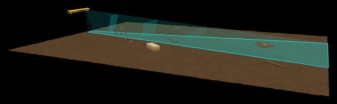
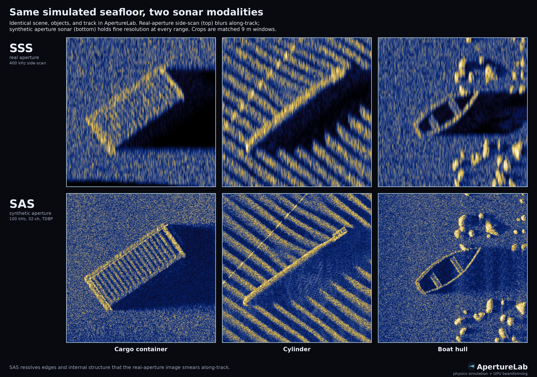
This appendix gives the point-scatterer acoustics in full: the observation model, the wavefront solver, the amplitude terms, shadowing, speckle statistics, calibration, and the GPU kernel that evaluates it.
A PoSSM-style coherent point-scatterer simulator; every ping is a time-domain sum of per-scatterer echoes, each carrying its own delay, amplitude, and carrier phase.
1. Observation model
For ping \(k\) on channel \(c\), the complex baseband pressure is a coherent sum over scatterers \(i\):
\[
s_{k,c}(t) \;=\; \sum_{i} a_{k,c,i}(t)\;p\!\left(t - \tau_{k,c,i}(t)\right)\;\exp\!\left(-j\,2\pi f_c\,\tau_{k,c,i}(t)\right),
\]
where \(p(\cdot)\) is the baseband LFM chirp, \(f_c\) is the carrier (300 kHz default), and
\[
\tau_{k,c,i}(t) \;=\; \frac{\lVert \mathbf{x}_i - \mathbf{x}^{TX}_k(t)\rVert \;+\; \lVert \mathbf{x}_i - \mathbf{x}^{RX}_{k,c}(t)\rVert}{c_s}
\]
is the bistatic two-way time between the TX phase center and the \(c\)-th RX element. Production runs are continuous-motion: the RX position is evaluated at the echo arrival time, not at ping start. Stop-and-hop is disabled by default and is forbidden in production imaging.
2. Wavefront–receiver intersection (the τ solver)
The bistatic arrival time \(\tau\) is not a closed-form quantity, because the receiver moves while the echo is in flight. The true \(\tau\) satisfies the implicit equation
\[
\tau \;=\; \frac{d_{TX} \;+\; \bigl\lVert \mathbf{x}_i - \mathbf{x}^{RX}(\tau)\bigr\rVert}{c_s},
\qquad \mathbf{x}^{RX}(\tau) \;=\; \mathbf{x}^{RX}_0 + \mathbf{v}\,\tau,
\]
i.e. \(\tau\) is the time at which the outgoing wavefront, after bouncing off the scatterer, intersects the receiver's straight-line trajectory. With the closed-form expansion of \(d_{RX}(\tau)^2\) along the trajectory,
\[
d_{RX}(\tau)^{2} \;=\; d_{RX}(0)^{2} \;-\; 2\,\tau\,\bigl(\mathbf{v}\!\cdot\!\Delta\mathbf{x}_{RX}\bigr) \;+\; \tau^{2}\,\lVert\mathbf{v}\rVert^{2},
\qquad \Delta\mathbf{x}_{RX} = \mathbf{x}_i - \mathbf{x}^{RX}_0,
\]
the implicit equation becomes a Picard fixed-point iteration, solved directly on the GPU:
\[
\tau^{(n+1)} \;=\; \frac{d_{TX} \;+\; \sqrt{\,d_{RX}(0)^{2} \;-\; 2\,\tau^{(n)}\,(\mathbf{v}\!\cdot\!\Delta\mathbf{x}_{RX}) \;+\; \tau^{(n)\,2}\,\lVert\mathbf{v}\rVert^{2}\,}}{c_s},
\qquad \tau^{(0)} \;=\; \frac{d_{TX}+d_{RX}(0)}{c_s}.
\]
The initial guess \(\tau^{(0)}\) is exactly the stop-and-hop delay. Each iteration is a contraction with rate \(\sim\!\lVert\mathbf{v}\rVert/c_s\), about \(10^{-3}\) at SAS speeds. One iteration therefore drops the residual TOF error from \(O(v R / c_s^{2})\) (sub-cm at 100 m range) into the noise floor of the FP64 carrier phase. The default is one iteration (\(\mathtt{PS\_N\_TOF\_ITERS}=1\)), chosen not for speed but to match the beamformer's \(\mathtt{n\_tof\_iters}=1\) MoComp model exactly. Simulator and beamformer use the same \(\tau\), so any residual phase error cancels coherently in TDBP rather than smearing the PSF.
Getting this delay wrong produces the asymmetric along-track sidelobe pattern of Cook & Brown (2009), the linear-phase-error signature of a stop-and-hop simulation driven through a continuous-motion beamformer. The solver above keeps that pattern out of the imagery.
3. Per-scatterer amplitude
The complex amplitude \(a_{k,c,i}\) factorizes (linear pressure, not intensity):
\[
a_{k,c,i} \;=\; \rho_i \cdot \underbrace{B_{TX}(\hat{\mathbf{u}}^{TX}_i)\,B_{RX}(\hat{\mathbf{u}}^{RX}_{c,i})}_{\text{rectangular-piston sinc}}\;\cdot\;\underbrace{\cos\theta_i^{n}}_{\text{Lambert}}\;\cdot\;\underbrace{\frac{1}{d_{TX,i}\,d_{RX,c,i}}}_{\text{two-way spreading}}\;\cdot\;\underbrace{e^{-\alpha(f_c)\,(d_{TX,i}+d_{RX,c,i})}}_{\text{Thorp absorption}}\;\cdot\;V_i.
\]
Each piston is a separable 2D sinc keyed on body-frame direction cosines, \(B(\hat{\mathbf{u}}) = |\mathrm{sinc}(\pi L_{az} u_x / \lambda)|\cdot|\mathrm{sinc}(\pi L_{el} u_z / \lambda)|\); attitude (R/P/Y) rotates the beam through \(R_{NED \to body}\). \(\cos\theta_i^{n} = |\hat{\mathbf{u}}^{TX}_i \!\cdot\! \hat{\mathbf{n}}_i|\) uses the heightfield surface normal at the scatterer: this is the Lambert directivity of Brown et al. 2019 (PoSSM). Per-scatterer reflectivities \(\rho_i = |\rho_i|\,e^{j\phi_i}\) carry Rayleigh-distributed magnitude with uniform phase. Absorption \(\alpha(f_c)\) is the Thorp seawater formula (~0.067 dB/m at 300 kHz).
4. Geometric shadows
The visibility factor \(V_i \in \{0,1\}\) (or a soft Fresnel knife-edge value in \([0,1]\) when enabled) comes from a DDA ray-march of the TX-to-scatterer segment against the heightfield: the ray is occluded at the first cell where \(z_{ray} > z_{terrain}\). Surface normals \(\hat{\mathbf{n}}_i\) are read from the same heightfield, clamped to a 60° max-slope so single-cell object edges cannot mute their surroundings.
5. Speckle and scatterer density
Scatterers are placed uniformly on the heightfield surface (with sub-wavelength normal-aligned jitter to avoid coherent halos). Per Goodman, fully-developed speckle requires \(N_{cell} \gg 1\) random complex scatterers per resolution cell; the bottom-type amplitude is calibrated by
\[
\sigma_z = \sqrt{\frac{\sigma_{bs}(20^\circ)}{2\,\rho\,\sin^2 20^\circ}},
\qquad \mathbb{E}[|\rho_i|] = \sigma_z\sqrt{\pi/2},
\]
where \(\rho\) is the scatterer density (m\(^{-2}\)) and \(\sigma_{bs}(20^\circ)\) is the APL-UW backscattering strength (e.g. \(-28\) dB for sand). The amplitude scaling absorbs \(\rho\) so the rendered intensity is density-invariant; \(\rho = 2000\)/m\(^2\) is the production working point, \(\rho = 200\)/m\(^2\) for debug.
6. Calibration constant
A deterministic calibration constant \(K_{PS}\) ties the simulator output to a closed-form analytic prediction for a known point target:
\[
|\text{peak}|^2_{\text{dB}} \;=\; TS \;-\; 40\log_{10}R \;-\; 2\alpha R \;+\; 10\log_{10}(BT),
\]
which combines two-way spreading, Thorp absorption, and the LFM matched-filter coherent gain \(10\log_{10}(BT)\). The calibration harness drives a single target through the full pipeline and asserts agreement to within ±1 dB.
7. GPU kernel
One CUDA thread per \((c, i)\) pair computes the carrier rotation \(e^{-j2\pi f_c \tau}\) in FP64, multiplies the pre-sampled chirp, and atomicAdds the result into an upsampled \((n_{ch}, K\!\cdot\!n_{samp})\) accumulator. The buffer is then FFT-domain low-passed and decimated to \(f_s\): the oversampling preserves sub-sample delay precision that would otherwise quantize to \(\pm 1/(2 f_s)\) range bins.