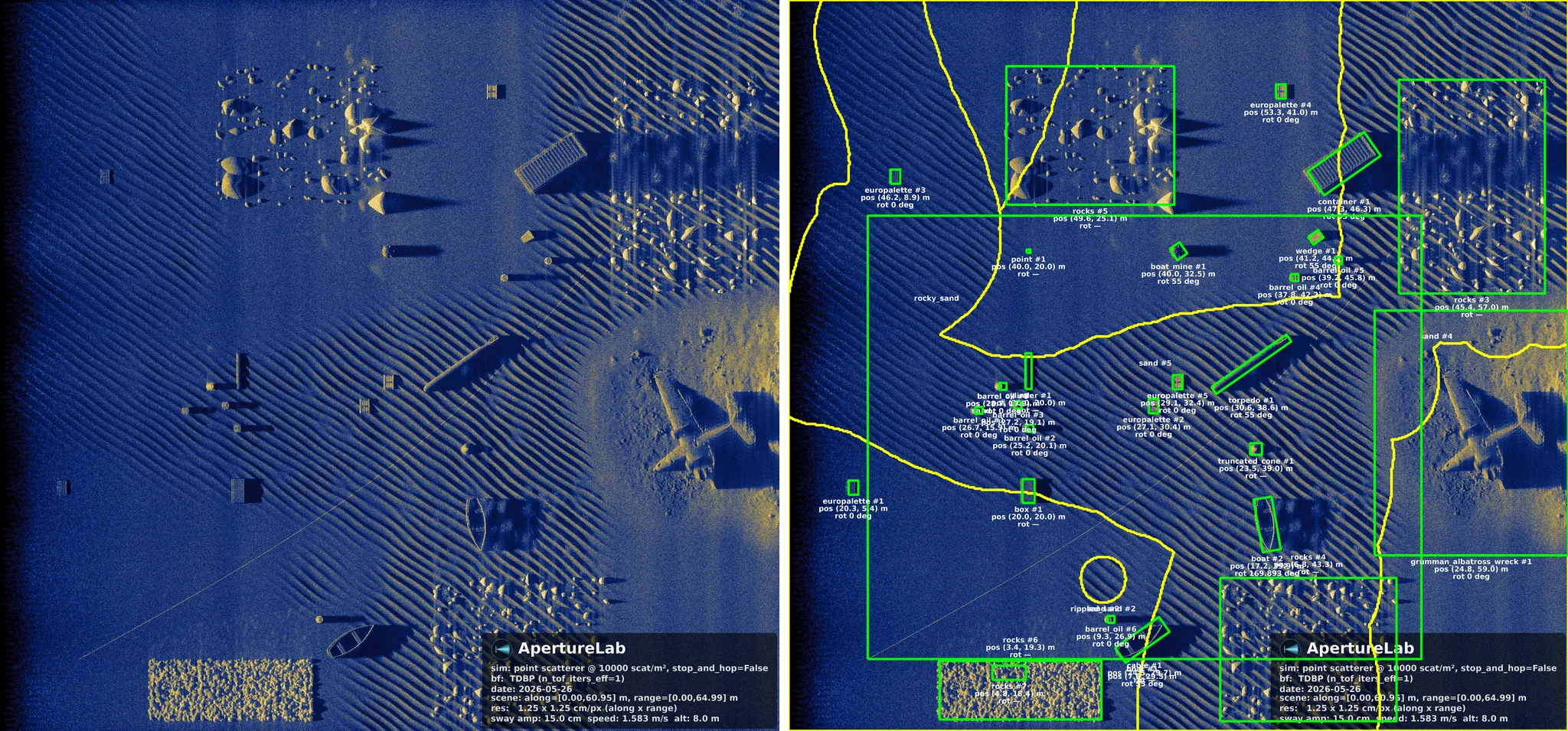
Every image arrives already labeled.

Labeled sonar imagery is scarce because labeling it is expensive: an analyst looks at a grey speckled scene and decides where an object ends and the seafloor begins. A simulator does not have that problem. It knows where everything is, because it put everything there. The labels are not inferred from the image; they are written out alongside it, from the same scene file the physics read.

Six annotation categories, in world coordinates.

Each simulated image is accompanied by annotations for objects, rocks, biota, pockmarks, trawl scars, and the seafloor itself. They are generated in world coordinates and projected into the image, so they stay correct when the geometry changes.

Objects get an oriented rectangle taken from the object's real footprint and heading, not an axis-aligned box fitted afterwards.

Cables and pipelines get a single buffered polyline per run, split at gaps and at heading breaks, so a pipeline that changes direction is one annotation rather than a chain of fragments.

Clutter fields (rocks, shells, biota) get a bounding region rather than thousands of unusable per-pebble boxes.

Seafloor types get a traced, Chaikin-smoothed outline per zone, taken from the zone raster the simulator actually rendered.

Burial is carried as a per-object property, so a partially buried target is distinguishable from an exposed one at training time.

Implementation: simulator/scenes/scene_annotations.py.

Standard COCO, with the geometry attached.

Annotations export as COCO detection JSON with polygon segmentation, which is what an off-the-shelf detector expects; there is no bespoke format to write a loader for. Each image record additionally carries pixel_size_m, along_extent_m, and range_extent_m, so a pixel box can be converted back into metres, and a georeference attached later, without re-deriving the imaging geometry.

Per-image files concatenate into one dataset with merge_coco(). A scene is a file, so a dataset is a parameter sweep over scene files; the cost of the next thousand images is the cost of the first one, times a thousand, with no ship.

A simulated synthetic aperture sonar scene beside the same scene overlaid with green object bounding boxes, object names and positions, and yellow traced seafloor-zone boundaries

One scene, imaged and labeled. Green: oriented object footprints with class, position, and heading. Yellow: the traced boundary of each seafloor type. Both are emitted by the scene file at simulation time.

Generators that have been run, and what they produced.

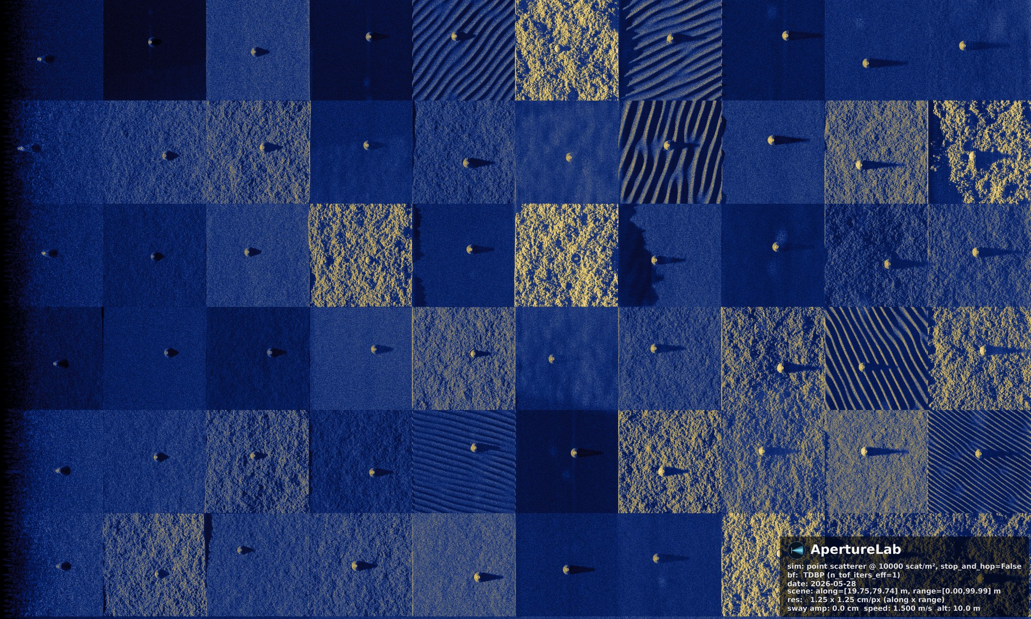
Five generators exist. Three have produced imagery with labels; two have produced the scene configurations an imagery run would consume. They are written here as what they are, not as a claim about scale that has not been exercised yet.

The public dataset: 1000 HISAS-class swaths with 2000 labeled targets and 2479 labeled clutter objects, COCO polygons and every scene file, on Hugging Face. See the dataset page.

A target-on-background grid: 60 instances of one object across ten distinct seafloor backgrounds, laid out so a 256 by 256 chip sits entirely inside one homogeneous background, with a per-instance CSV manifest.

Change-detection pairs: scene configurations for the same patch before and after, pixel-registered by construction, with heightmap previews rendered for review. The imagery has not been simulated yet.

Linear-feature pilot: 20 simulated scenes of pipes and cables with varying burial, constrained so runs never intersect, which is how real subsea infrastructure is routed.

A 151-scene ocean archetype library: scene configurations rather than rendered imagery, covering wrecks, pipelines, debris fields, trawl scars and pockmarks, each parametric and reseedable.

A grid of identical targets rendered against ten different seafloor types including fine ripple, coarse ripple, rocky, mud, and gravel

The same object on ten seafloor types. Domain randomization is not a post-process here; each background is a different physical bottom, simulated.

The same physics that renders a labeled scene forward is what trains the model that reads one backward.