ApertureLab · Performance

How long does one image take?

A synthetic aperture image is not free. Every pulse has to be propagated to a seafloor made of millions of individual reflectors and back, and then hundreds of pings have to be coherently focused into a picture. This page measures that, end to end, and compares it with the time the sonar spent gathering the data in the first place.

One scene, held fixed.

Everything below images the same patch of seafloor from the same trajectory. The platform flies a curved track that loops around the scene rather than past it, so objects are lit from many aspects and their shadows fall in different directions.

71 × 100 m

seafloor simulated, 7,145 m²

380

pings along a Catmull-Rom spline track

2.5 cm

image pixel, in both range and along track

134 s

the sonar's own collection time, at 2.83 pings per second

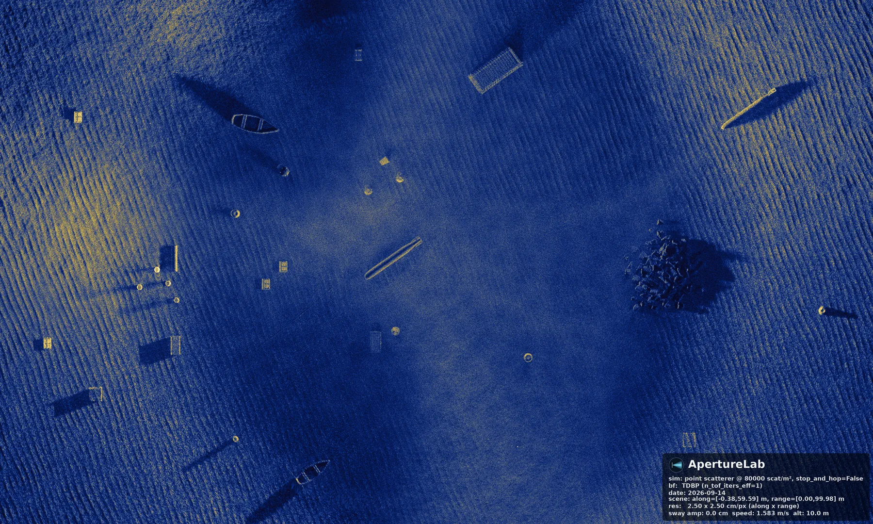
A simulated synthetic aperture sonar image of a seafloor scene holding boat hulls, a torpedo shape, containers, barrels, truss frames and a rock outcrop over rippled sand

The scene at 80,000 scatterers per square metre. Shadows point in several directions because the aperture curves around the objects rather than passing them on one side.

What density buys you.

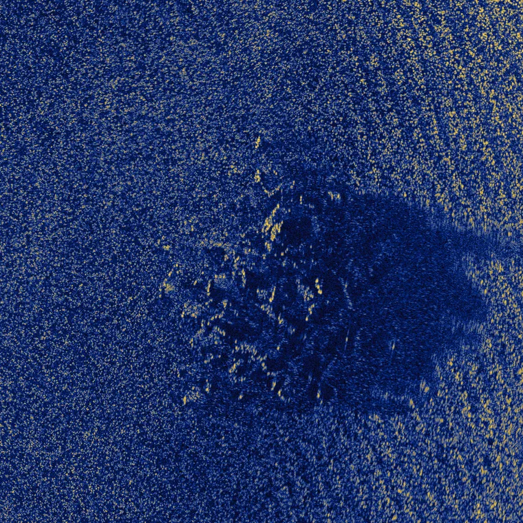
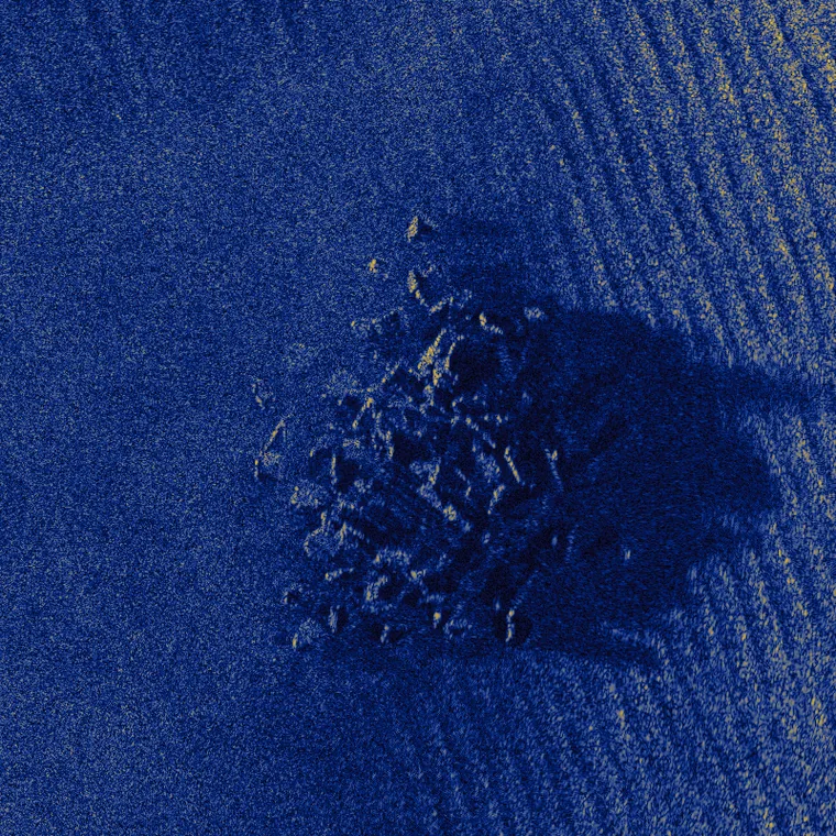
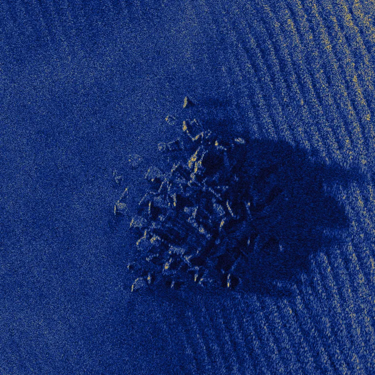
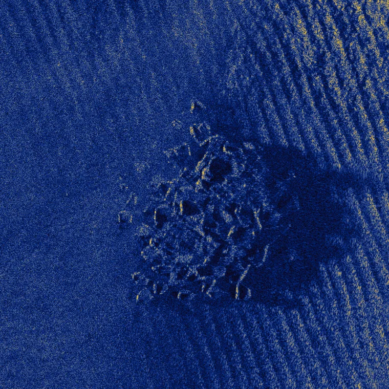
Scatterer density sets how finely the seafloor is discretised. Too few reflectors per resolution cell and the speckle is not fully developed: the image looks grainy in a way real sonar does not, and fine relief breaks up. Past a point the returns are already statistically converged and more reflectors buy nothing but time.

The same 20 m square of one scene, a rock outcrop with its acoustic shadow beside a ripple field, at four densities. Click any tile to enlarge it.

A rock outcrop and its acoustic shadow on rippled sand, simulated at 200 scatterers per square metre — **200/m²** 1 M scatterers · 73 s

A rock outcrop and its acoustic shadow on rippled sand, simulated at 2,000 scatterers per square metre — **2,000/m²** 14 M scatterers · 80 s

A rock outcrop and its acoustic shadow on rippled sand, simulated at 20,000 scatterers per square metre — **20,000/m²** 143 M scatterers · 145 s

A rock outcrop and its acoustic shadow on rippled sand, simulated at 80,000 scatterers per square metre — **80,000/m²** 572 M scatterers · 20.5 min

The jump from 200 to 2,000 per square metre is the one that matters; beyond roughly 20,000/m² the differences are subtle and the cost is not.

Time to form one image.

The whole path a user waits through: scene build, point-scatterer simulation, back-projection, and writing the output image. Nothing is cached; every point re-simulates from the scene file. Measured on NVIDIA RTX 4500 Ada, 24 GB.

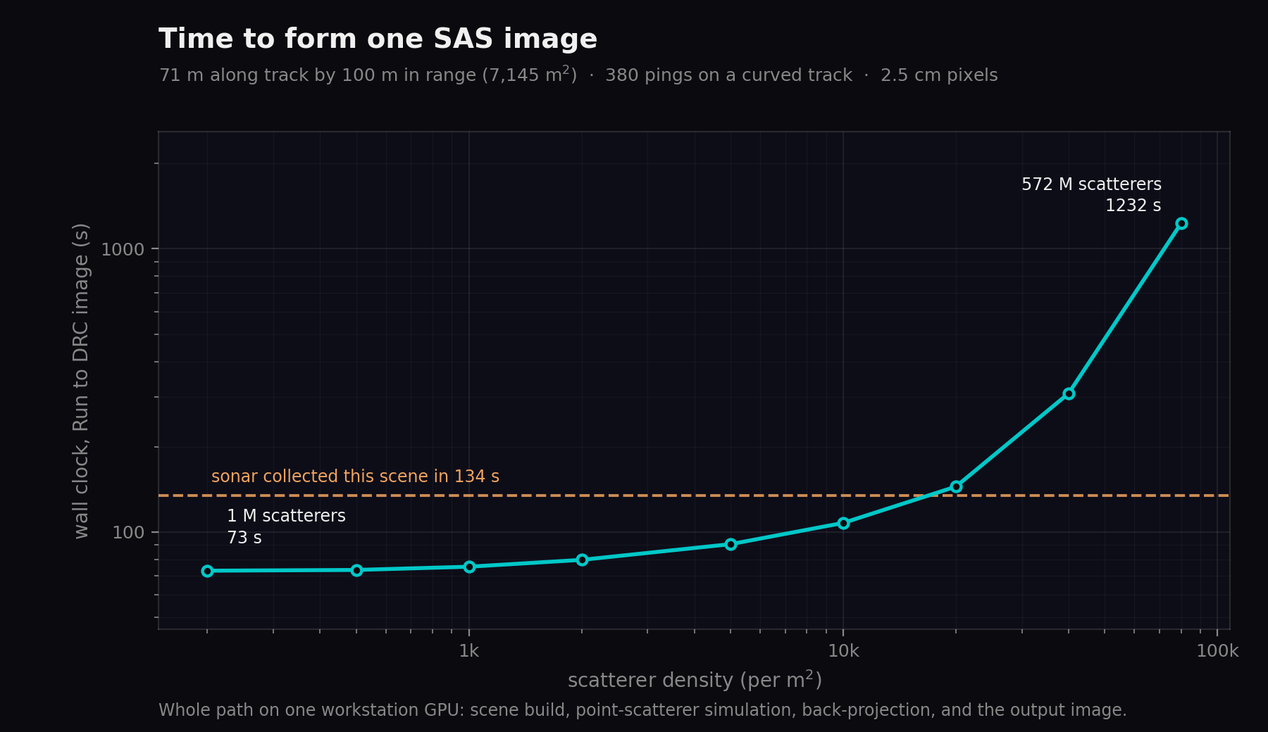
Below about 2,000 scatterers per square metre the wall clock barely moves, because fixed costs rather than the physics dominate: at 200/m² the run takes 73 s. Past that the scatterer count leads, and at 80,000/m², which is 572 million reflectors, the same image takes 20.5 min.

Wall clock to form one image against scatterer density on log axes, flat near 73 seconds up to about 2,000 per square metre and rising to 1232 seconds at 80,000 per square metre, with a dashed line marking the sonar's 134 second collection time

The dashed line is the sonar's own collection time. Where the curve sits below it, the workstation formed the image faster than the platform gathered the data.

Faster than the sonar, up to a point.

The sonar spent 134 s flying this track and listening. A real-time factor above 1 means the workstation produced the finished image in less time than that.

The crossover sits near 16,821 scatterers per square metre. Below it, one workstation forms the image faster than the sonar gathered the data; above it, the physics costs more than the collection did.

density	scatterers	wall clock	vs real time
200	1.4 M	73 s	1.84x
500	3.6 M	74 s	1.83x
1,000	7.1 M	75 s	1.78x
2,000	14.3 M	80 s	1.68x
5,000	35.7 M	91 s	1.48x
10,000	71.5 M	108 s	1.25x
20,000	142.9 M	145 s	0.93x
40,000	285.8 M	5.1 min	0.44x
80,000	571.6 M	20.5 min	0.11x

density

scatterers

wall clock

vs real time

200

1.4 M

73 s

1.84x

500

3.6 M

74 s

1.83x

1,000

7.1 M

75 s

1.78x

2,000

14.3 M

80 s

1.68x

5,000

35.7 M

91 s

1.48x

10,000

71.5 M

108 s

1.25x

20,000

142.9 M

145 s

0.93x

40,000

285.8 M

5.1 min

0.44x

80,000

571.6 M

20.5 min

0.11x

From 40,000 to 80,000 per square metre the scatterer count doubles but the wall clock grows by 4.0x. Past roughly half a billion reflectors something other than arithmetic is binding; host memory is the suspect, and it is the next thing to profile.

How these were measured.

One density per process, so one point's memory pressure cannot distort the next.

Simulation forced on every run. A cache hit would measure the cache, not the simulator.

Timer starts where a user presses Run and stops when the image is on disk, so scene build and file writing are included, not just the GPU kernels.

Ascending density, so a failure at the top still leaves a usable curve.

The scene is frozen in the repository as a benchmark fixture, and the numbers on this page are read from the results file at build time rather than typed in.