A seafloor you can author, seed, and regenerate.

A scene names the seafloor, the objects on it, the vehicle's motion, the sonar, and the products to write. Scenes inherit from each other, so a variation is a short file rather than a copy. A profile bundle can carry two imaging configurations at once, which is how the same seabed gets rendered as both a synthetic-aperture collection and a real-aperture side-scan line without a second scene.

Six bottom types ship built in (sand, rippled sand, mud, rock, gravel, silt), each calibrated to a measured backscattering strength, and a scene can define its own. Objects come from a catalogue of 69 placeable models, plus procedural rock and biota generators.

The tell of a synthetic seabed is straight lines where nature has none: a ripple field that stops dead on a grid boundary, a sediment patch with corners, a roughness change along a raster edge. A model trained on that learns the artifact.

Seafloor zones are painted as a raster and then blended with a warped, feathered boundary, so a bottom-type change follows an irregular line and the roughness crossfades across it. The feather runs inward from the boundary rather than outward, which is what keeps a ripple patch from bleeding into its neighbour. Seam quality is scored in the test suite across all fifteen pairs of bottom types.

The features themselves follow published morphology rather than taste: ripple geometry after Tang et al. 2009, pockmarks after Hovland and Judd, seabed roughness after Goff and Jordan, and burial and scour from Shields-criterion sediment mechanics, so a partially buried object sits at a depth the sediment and current would actually produce.

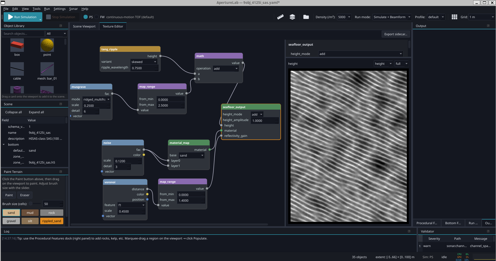
Seafloor texture is authored the way a Blender artist builds a material: as a graph of nodes. Seventeen node types (fractal noise, multifractal, Voronoi in several modes, the Tang ripple model, power-law roughness, pockmark and rock scatter, plus the usual maths and mixing operators) drive four channels at once: the bathymetry, the bottom-type map, a per-cell backscatter gain, and rock placement.

The noise is pure integer hash, so a graph evaluates identically at any resolution, on CPU or GPU, from the same seed. That is the property that matters for training data: a recipe is a reproducible distribution, not a one-off asset. One graph reseeds into thousands of statistically distinct seafloors, and a scene that produced a surprising result can be regenerated exactly.

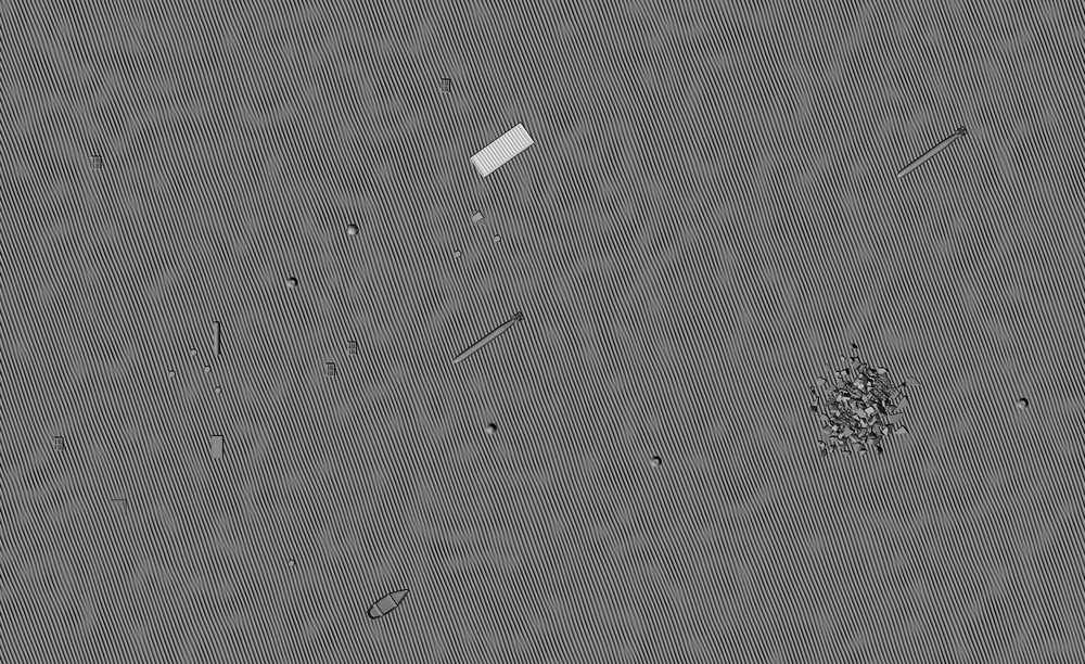
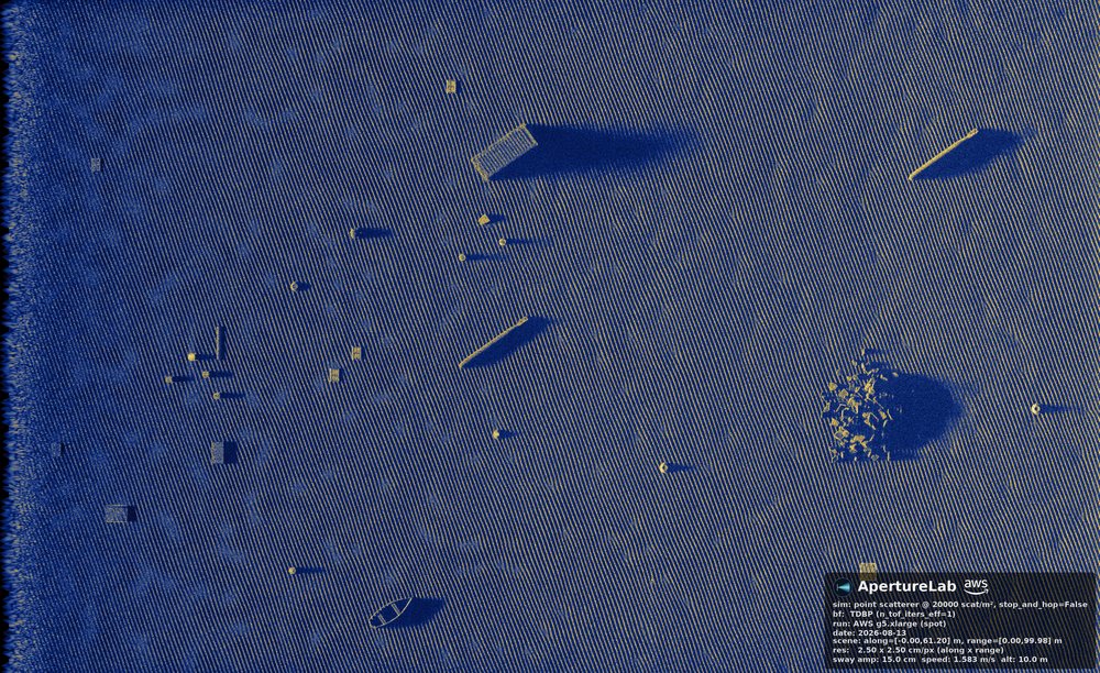
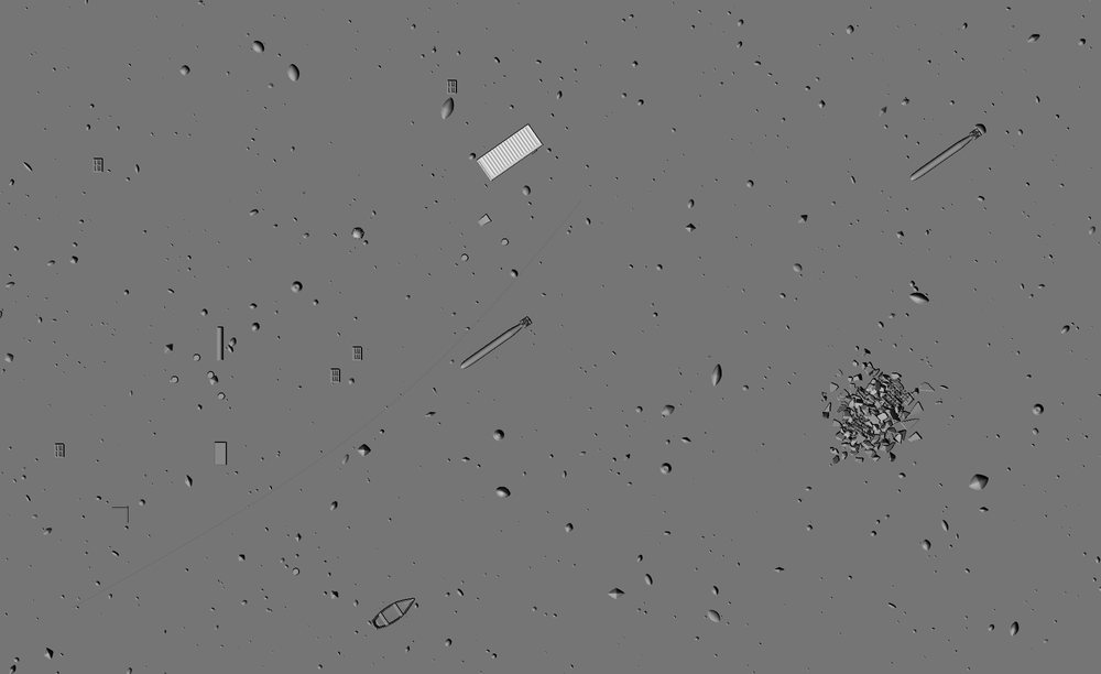
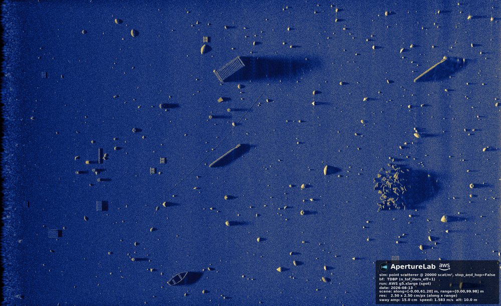
Each pair below is one seafloor twice: the heightfield the scene defines, and the sonar image the physics produces from it, at matched framing. The left is not a derived product of the right; it is the input. That relationship is what makes every downstream label exact rather than estimated.