Raw returns are not a picture.

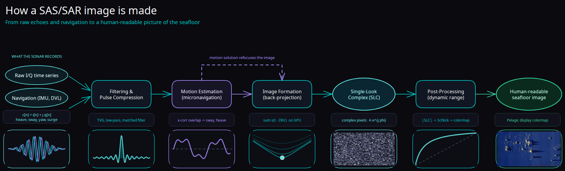
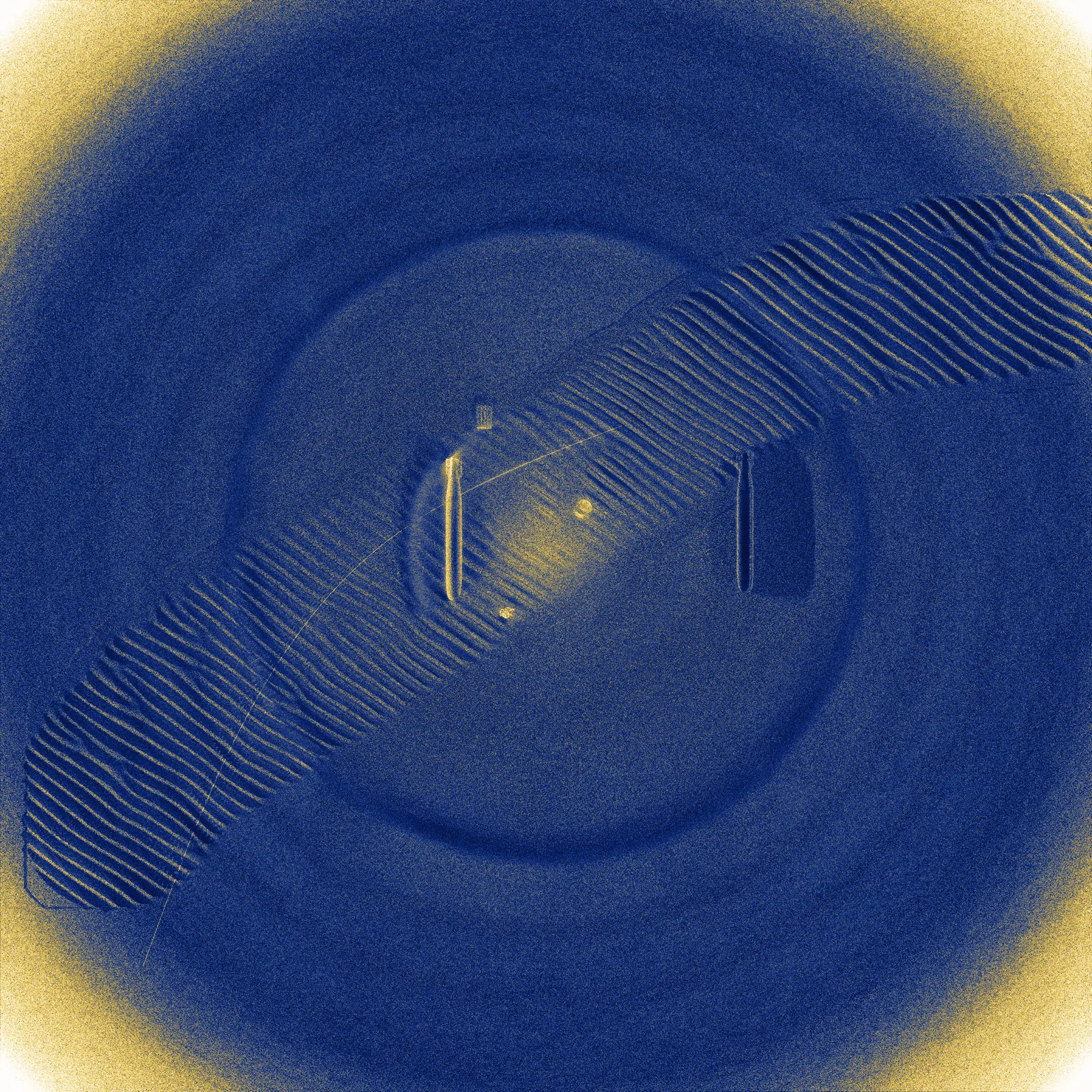
A sonar does not take photographs. What comes off the array is a complex time series per channel per ping: pressure against time, with no image in it. The image is constructed afterwards, by asserting where the platform was when each of those returns was recorded and summing them so that energy from the same patch of seabed arrives in phase. Get the platform position wrong by a fraction of a wavelength and the image blurs.

From a raw cube to a focused scene.

The pipeline runs in a fixed order, and each stage is checkable against the file's own recorded attributes rather than against an assumption made at the top.

Load the raw cube and check it against the physics the file declares: sound speed, sample rate, array geometry.

Zero-phase lowpass, then matched filtering, which compresses each long transmitted chirp into a sharp pulse and is where range resolution comes from.

Cross-ping time-varying gain, so returns from 90 m are comparable to returns from 10 m, and glint suppression for specular flashes that would otherwise dominate the dynamic range.

Eight-times range upsampling, so the back-projection can interpolate without quantising delay.

Micronavigation, which measures where the platform actually went.

Time-domain back-projection on the GPU, producing a single-look complex image on a georeferenced grid.

Dynamic-range compression for viewing.

A left-to-right pipeline diagram titled How a SAS/SAR image is made. Raw I/Q time-series and navigation feed into filtering and pulse compression, then motion estimation by micronavigation, then image formation by back-projection, producing a single-look complex image, then post-processing for dynamic range, ending in a human-readable seafloor image. Each stage shows a small example of its data: I/Q traces, a compressed pulse, an estimated sway track, focusing arcs, complex speckle, a tone curve, and a real focused sonar image.

The same chain as a figure, from raw I/Q and navigation to a focused seafloor image, with each stage shown carrying its own data at that point in the chain.

Back-projection, wavenumber, and real aperture.

Time-domain back-projection is the production path. It makes no assumption that the platform flew straight: it handles continuous motion, six-degree-of-freedom attitude, curved tracks, and circular collections, and because it is geometry-driven rather than band-specific it also focuses airborne radar.

Wavenumber (omega-k) processing is the exact inverse of the Fourier-wavefield forward model, which makes the pair a useful consistency check on each other, at the cost of assuming stop-and-hop motion.

Real-aperture stacking forms conventional side-scan imagery, so one scene can be compared across both imaging regimes.

9.6 Mpx in 9.6 s

a 2400 by 4000 pixel image at 2.5 cm, against 134 s of collection time; roughly fourteen times faster than the sonar gathers it

.gui-imgui.log, 2026-09-13

Measuring the track from the echoes themselves.

Inertial navigation is not accurate enough to focus a synthetic aperture. At 300 kHz the wavelength is 5 mm, and the platform position has to be known to a small fraction of that over an aperture several metres long. No affordable instrument delivers it.

So the track is recovered from the data. Every ping lays down a row of phase centres, the transmitter-receiver midpoints, spaced half a channel apart; the vehicle advances a whole number of those spacings between pings, two short of the array, so consecutive pings share two phase centres. On the instrument the fidelity page measures, that is 36 phase centres per ping and an advance of 34 spacings: the two fore-most centres of one ping are re-occupied by the two aft-most of the next. Those repeated centres observed the same patch of seabed from the same place, so comparing the phase of the two recordings measures how far the vehicle really moved, not how far it was commanded to. Those per-pair delay estimates are then fitted, with a Huber-robust least squares that keeps a handful of bad correlations from dragging the whole track, into a per-ping sway and heave history that the beamformer uses instead of the nominal line.

Even a perfectly measured track leaves one error behind: it corrects the path exactly only for points on the surface being imaged. How motion then blurs objects that stand above that surface is shown interactively in The surface of focus.

< 0.625 mm

fine delay error at 300 kHz, one eighth of a wavelength, asserted in the test suite at correlation above 0.9

beamformer/tests/test_delay_estimation.py

You can see this fail on purpose: the sound-speed slider on the walkthrough page introduces exactly this kind of error and blurs the image in front of you.

What you look at, and what you process.

The beamformer's real output is the single-look complex image: phase intact, suitable for coherent change detection, interferometry, and sub-aperture analysis. That is the product to train on.

The picture is derived from it for human eyes: magnitude, an adaptive Schlick tone map to pull a very large dynamic range into a displayable one, and a perceptual colour map. There is no logarithm in that chain, which matters if you are reproducing the display or comparing levels against it.

A circular-collection synthetic aperture sonar image: a bright ring around a dark disc with ripple structure crossing the centre

A circular collection, 360 degrees around one point. Back-projection does not care that the track is not a line, so every facet of a target is resolved from some aspect.