ApertureLab scenes run unchanged on cloud GPU instances: the same YAML that renders on a workstation becomes a batch of self-managing spot instances, one machine per scene. A ten-scene set finishes in roughly the time of one. This page covers what a scene is and what it costs, how a batch runs, and the tooling that keeps spend as disciplined as the physics.
Scale, speed, cost
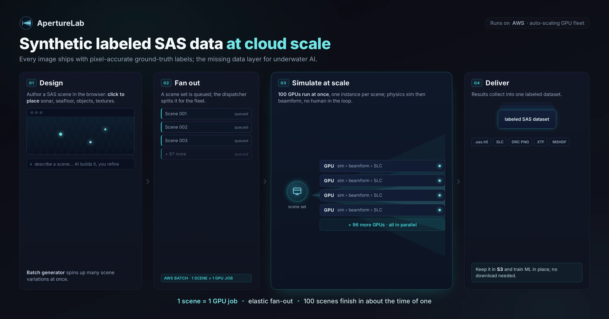
The unit of work is a complete scene, simulated and beamformed at production fidelity; not a crop, not a preview.
These are initial numbers and likely to change. They dropped roughly 10x in one day of optimization (an FFT-based rewrite of the echo-accumulation kernel) and are expected to keep moving as the pipeline is profiled further.
The mechanism
One command submits a batch: python -m cloud run
<scene>.yaml, or the Run on AWS button in the GUI. Code
ships content-addressed; a given version uploads once, not once per
job, so submitting fifty scenes moves fifty small scene files and zero
redundant copies of the codebase. From there each job is on its own.
Each job gets its own spot GPU instance. A launch loop fills however many quota slots exist, hunts across availability zones for spot capacity cheapest-zone-first, and retries transient capacity droughts indefinitely; a batch submitted into a dry market simply waits and fills as capacity appears.
The instance boots, pulls the worker container, and unpacks the content-addressed code snapshot for the submitted version.
The full pipeline runs on the instance's GPU: acoustic simulation to complex IQ, then time-domain back-projection to a focused, georeferenced image, identical to a local run of the same scene file.
Products upload to S3 and the instance terminates itself. Results stream back to the CLI or GUI exactly as a local run would; closing the GUI does not kill the job.
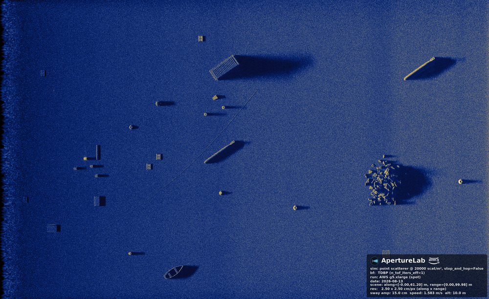
Every image carries its provenance: a watermark records the instance type and whether it ran on spot or on-demand capacity, so cloud-generated imagery is always identifiable as such and traceable to the hardware that produced it.
Setup
Setup is a single idempotent command: python -m cloud
init creates the storage bucket, the worker role, and the
network configuration in your own AWS account, everything tagged so it
can be found and removed as a unit. The worker container image is
public. After that, a scene runs from one CLI command or from the Run
on AWS button next to Run in the GUI; progress, logs, and products
land in the same panels as a local run.
Monitoring
Elastic compute is only useful if it cannot surprise you. The cloud path treats cost the way the simulator treats physics: measured, bounded, and checked at every step rather than assumed.
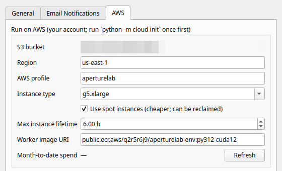
The AWS tab in the workbench: per-job status and live cost estimates while jobs run, with month-to-date billed spend one click away.
The rigor applied to the acoustics is applied to the invoice; both are part of making synthetic SAS data cheap enough to treat as an AI modality.
Preflight
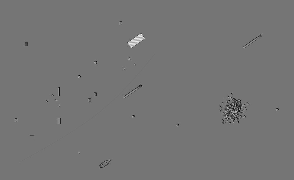
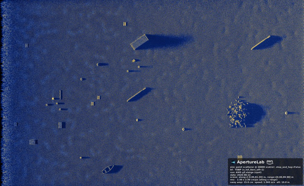
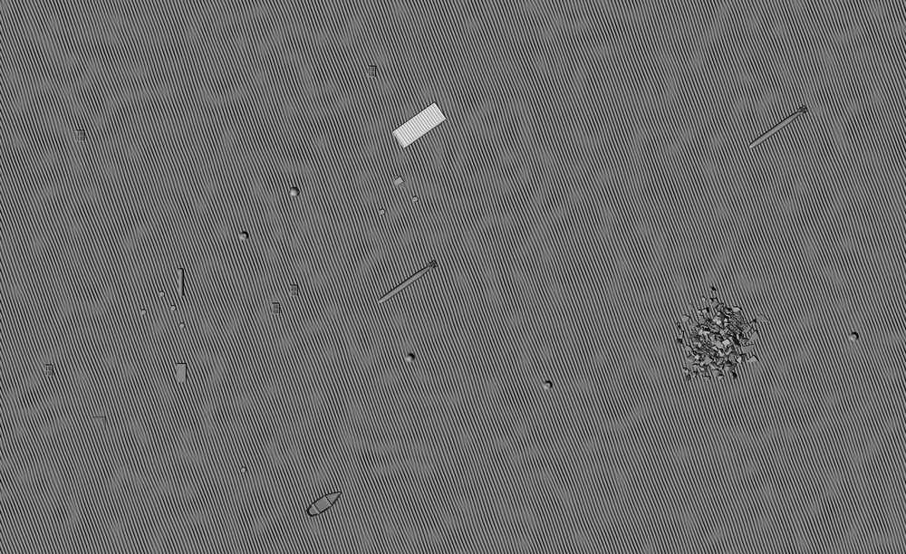
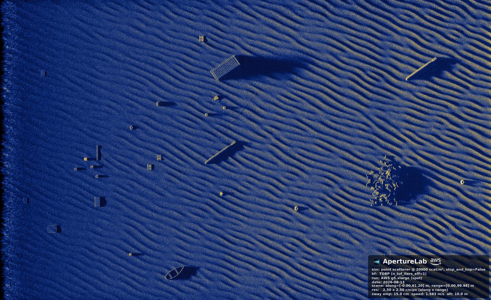
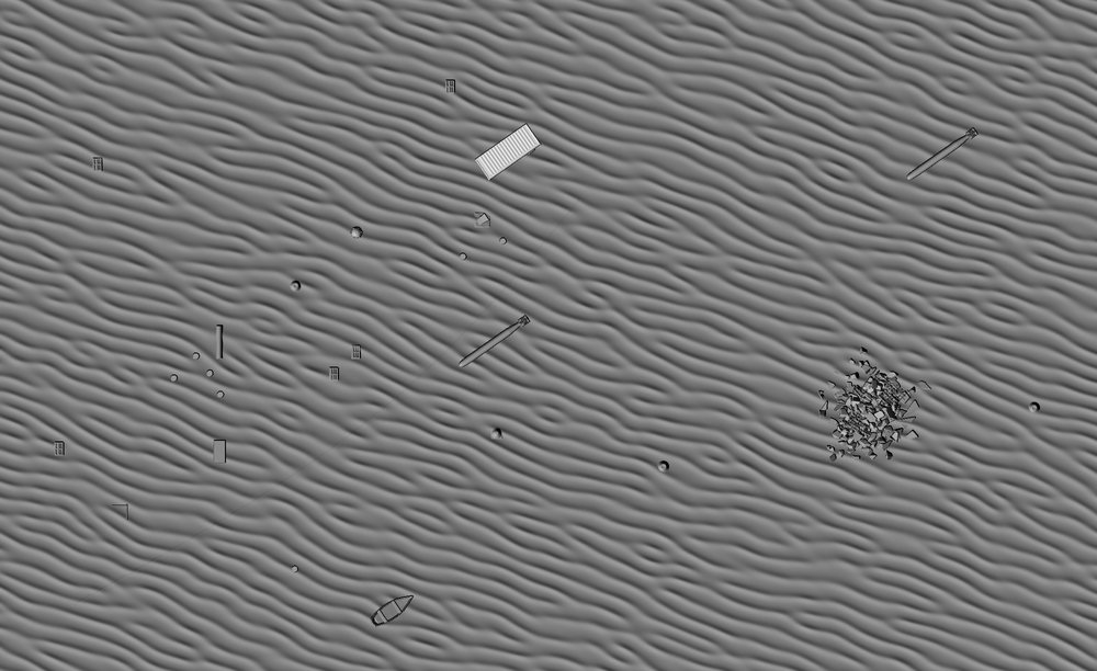
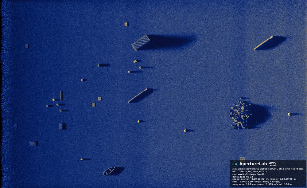
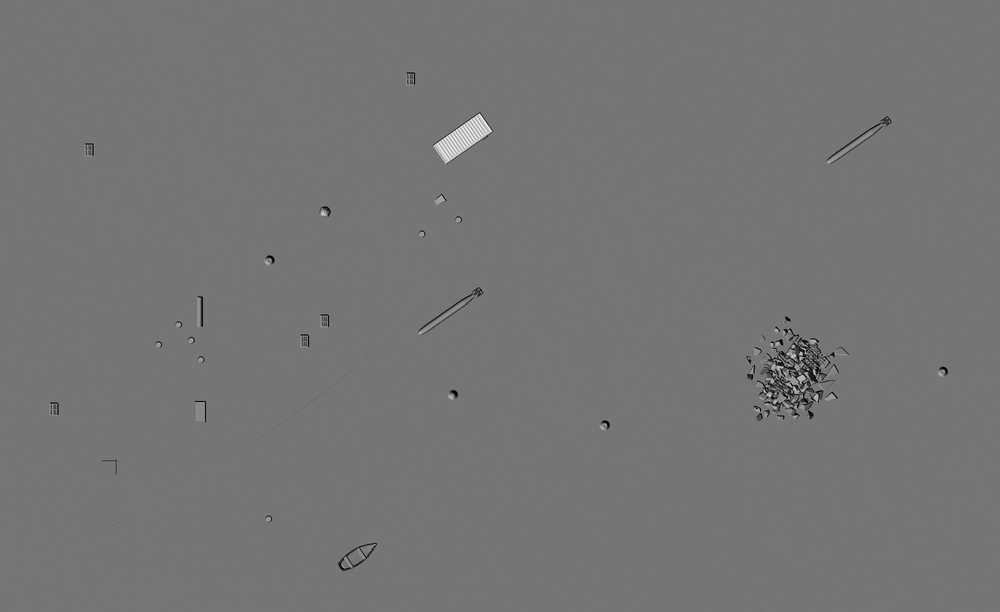
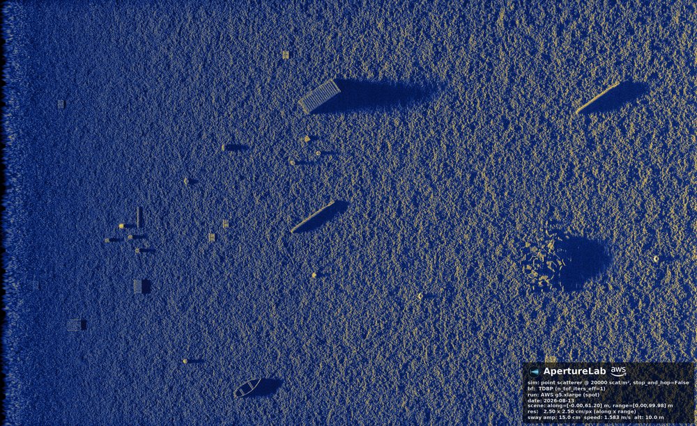
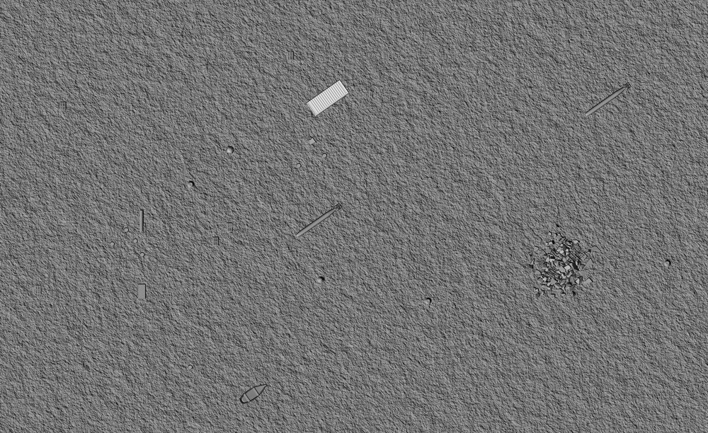
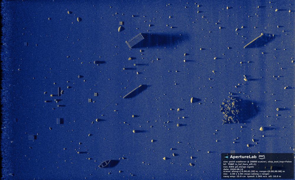
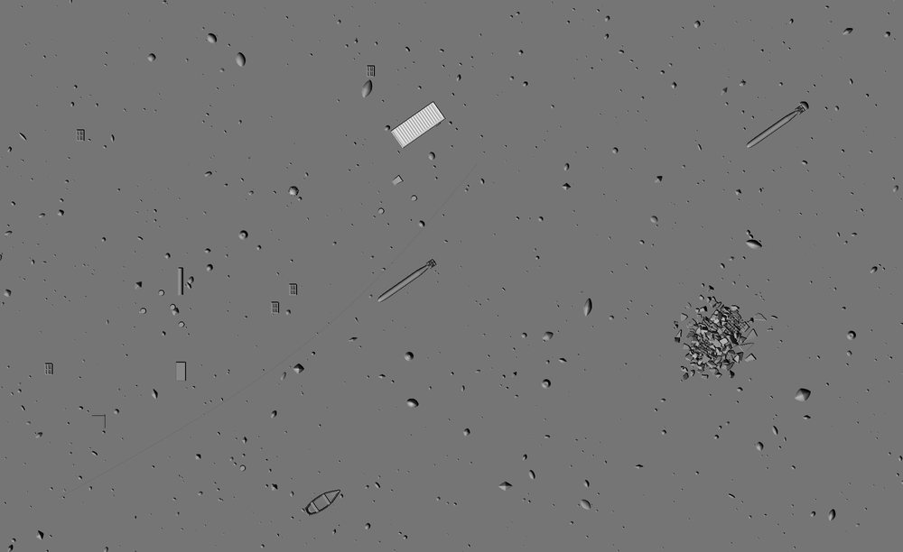
Before a batch launches, the scene's heightmap renders locally in about 30 seconds, for free: seafloor zones, ripple fields, and object placement on the exact geometry the simulator will trace. Approve it, then let the cloud make the real image. The six tiles below are the six scenes generated on the cloud so far; each one crossfades between its local heightmap preflight and the cloud-rendered SAS image. The geometry is identical, so the two fade into alignment.
Sand
Fine ripple
Coarse ripple
Mud
Fractal
Rocky
Six seafloor types, each proofed as a free 30-second local heightmap before its 20-minute cloud render. Pixel registration between the pairs is exact; what you approve is what the physics images.