ApertureLab Synthetic SAS Dataset, version 1.1.

A labeled dataset earns trust through its labels and its variety. The first release showed that a thousand simulated sonar swaths could be produced and labeled on one workstation; an audit of it also showed where it fell short: labels that did not follow burial or terrain, a flat seafloor with only centimetres of relief, one acquisition geometry, and an information box burned into every image. Version 1.1 re-issues the same thousand-swath footprint with those faults corrected, labels four target shapes and 23 kinds of clutter, each as its own category, and adds the terrain and boulder tables that let a scientist check an image against what produced it.

It is being regenerated. A first render under an earlier four-category label scheme was stopped and withdrawn from Hugging Face; the regeneration labels every object kind as its own category, as described below, starting with a 20-swath pilot and then the full batch. The dataset card, with counts read from the finished files, will follow when all 1000 swaths are complete. The other release is described on the Datasets page.

Status

Regenerating, labelled by object kind.

Status
Regenerating The 20-swath pilot has rendered. The full batch of 1000 was restarted on the evening of 2026-09-23 so that every label file is written in the per-kind categories; the figures on this page are drawn from swaths of the first run, which rendered the same scenes with the same renderer.
Rendered at
Commit 3d7efa5, recorded as git_sha in every label file. The first swath, si_0000, records bf0e096, which differs from it only in website files.
Repository
huggingface.co/datasets/idg101/Aperture_Lab_Synthetic_Aperture_Sonar_v1_1
License
ALSD-1.0, the ApertureLab Synthetic SAS Dataset License, unchanged from v1.0.

The whole release is rendered at commit 3d7efa5, which includes the beamformer and seafloor corrections validated against published physics on the Fidelity page.

Changes from v1.0

What was corrected, and what was added.

The footprint of a swath is unchanged: 200 m of ground range by 80 m along track at 2.5 cm, from the same HISAS 1030 preset. Every scene is drawn fresh from a new master seed. The differences are these:

Label classes

Four target shapes and 23 kinds of clutter.

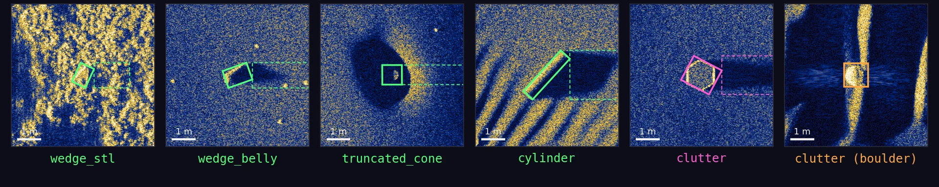
A detector trained on this set has to tell four target shapes apart and separate all of them from everything else that returns an echo from the seafloor. The figure shows one labelled example of each target class and two of the clutter categories, a boulder and a placed object, each cropped from a regenerated swath around its COCO box.

Six sonar chips in a row, each 6 m square with its label polygon drawn and its category name below: wedge_stl, wedge_belly, truncated_cone, cylinder, a placed clutter object and a boulder (rock)
Each target class and two clutter categories6 m chips at the native 2.5 cm, cropped around the COCO box, with the footprint polygon solid and the shadow polygon dashed; targets in green, a placed clutter object in magenta and a boulder in orange; a 1 m bar in each corner
1 wedge_stl
Target: a wedge resting level with its base sunk into the bed, so only its upper part stands proud.
2 wedge_belly
Target: the same wedge lying on its flat underside, standing higher off the bed and casting a longer shadow.
3 truncated_cone
Target: a truncated cone standing on its base.
4 cylinder
Target: a cylinder lying on its side.
5 rock
Clutter: every simulated boulder of 0.75 m diameter or more from the rocks CSV, labelled individually; smaller boulders stay in the CSV only.
6 to 17
Clutter, parametric shapes: pyramid, cone, frustum, dome, drum, slab, hexprism, capsule, cross, polyhedron, mound, torus.
18 to 27
Clutter, meshes: tire, barrel_oil, keg, sunken_anchor, fish_trap_square, ladder, debris1, ship_propeller, europalette, rock_pile.
28 clutter_other
Reserved for clutter kinds outside this dataset, such as a user's own mesh in an ApertureLab scene; it never occurs in v1.1.

Every target carries its footprint polygon shrunk by burial, a shadow polygon, and its bed height, grazing angle, substrate and range band as attributes. Categories 1 to 4 share the supercategory target and categories 5 to 28 share the supercategory clutter, so a detector can be trained on the two supercategories or on every kind. The ids are fixed: a kind that never appears in a swath keeps its id. Every clutter annotation also keeps its kind in attributes.shape and its origin, rock_field or placed_object, in attributes.source. Seafloor features that are not objects, such as ripple zones, bathymetry operators, trawl scars, pockmarks and outcrops, are recorded with their parameters in the image record rather than drawn as boxes. Every target and clutter object is placed at least 1.5 m inside the image, so no label is clipped by an edge.

classtrainvaltesttotal
Targets
wedge_stlTBDTBDTBDTBD
wedge_bellyTBDTBDTBDTBD
truncated_coneTBDTBDTBDTBD
cylinderTBDTBDTBDTBD
targets, 4 classesTBDTBDTBDTBD
Clutter
rockTBDTBDTBDTBD
pyramidTBDTBDTBDTBD
coneTBDTBDTBDTBD
frustumTBDTBDTBDTBD
domeTBDTBDTBDTBD
drumTBDTBDTBDTBD
slabTBDTBDTBDTBD
hexprismTBDTBDTBDTBD
capsuleTBDTBDTBDTBD
crossTBDTBDTBDTBD
polyhedronTBDTBDTBDTBD
moundTBDTBDTBDTBD
torusTBDTBDTBDTBD
tireTBDTBDTBDTBD
barrel_oilTBDTBDTBDTBD
kegTBDTBDTBDTBD
sunken_anchorTBDTBDTBDTBD
fish_trap_squareTBDTBDTBDTBD
ladderTBDTBDTBDTBD
debris1TBDTBDTBDTBD
ship_propellerTBDTBDTBDTBD
europaletteTBDTBDTBDTBD
rock_pileTBDTBDTBDTBD
clutter_othernot usednot usednot usednot used
clutter, 23 classesTBDTBDTBDTBD
all labels, 27 classesTBDTBDTBDTBD

TBD: the counts are read from the label files when the full batch has finished rendering.

The products of one swath

Five files per swath, shown for three seafloors.

Every figure below is drawn from the files of a regenerated swath at 10 000 scatterers per square metre by tools/build_datasets_figures.py, exactly as they are downloaded; the scene name and its seafloor family are printed in the corner of each figure. The three scenes were chosen so that together they hold every label class. All share the house orientation: along track up, range to the right, the first row of each file at the top.

*_tdbp_drc.tif
The image: 8000 by 3200 px, 8-bit palette GeoTIFF with the 256-entry ApertureLab sonar palette and deflate compression. A reader that ignores the palette gets the grey display image.
*_tdbp_coco.json
The labels in the 27 categories, and in its image record the acquisition (altitude, sound speed, noise, residual motion), the tone map, the scene's features, the sibling products and the commit.
*_dem.png
The composed seafloor as a 16-bit PNG on 5 cm cells, after bathymetry, roughness, ripples, objects and scour: height in metres is v / 65535 × (z_max_m − z_min_m) + z_min_m, with both constants in the file's own metadata.
*_rocks.csv
One row per simulated boulder: group, position, bed height, diameter, target strength and burial.
scenes/*.yaml
The scene that produced the swath, editable and re-runnable in ApertureLab.

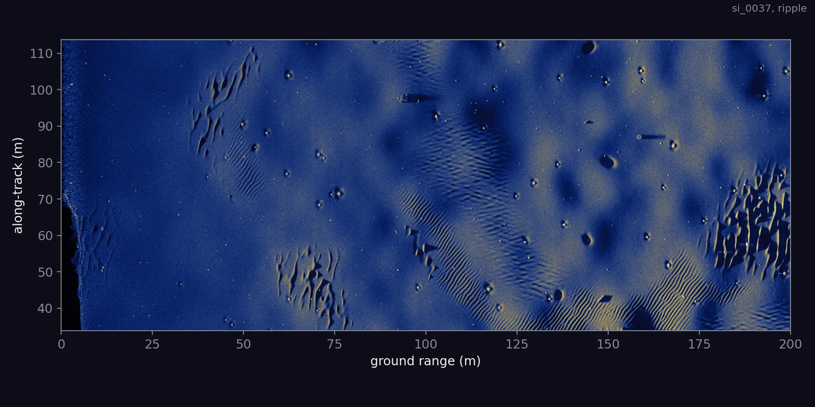
Rippled sand

Whole v1.1 swath of a rippled sand seafloor
The imagethe whole swath, reduced from 8000 by 3200 px
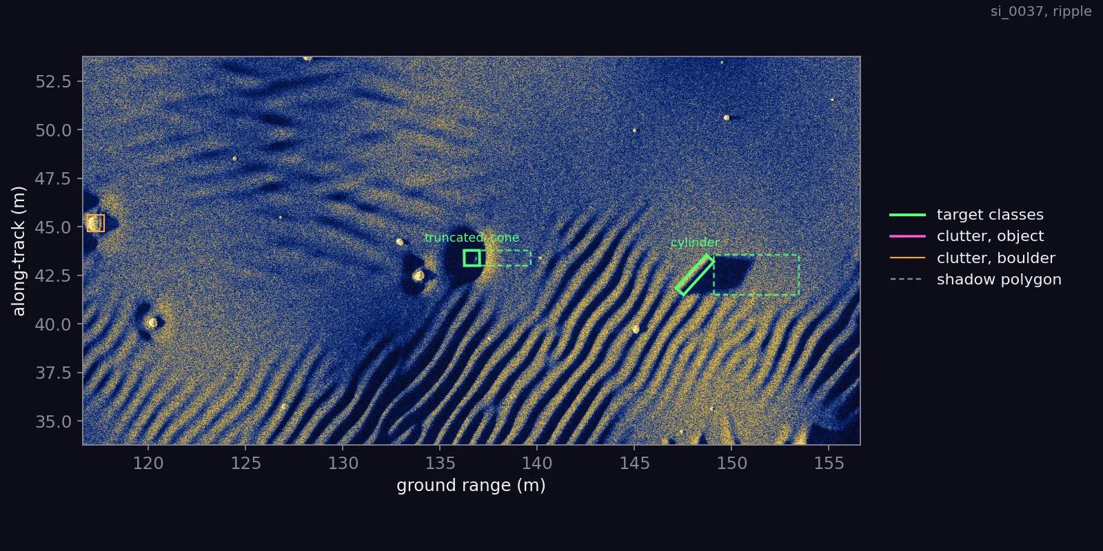
A 40 m by 20 m window of the swath at full resolution with its label polygons drawn
A window, labelled40 m by 20 m at full resolution; target classes in green with their names, clutter objects in magenta, boulders in orange, shadow polygons dashed
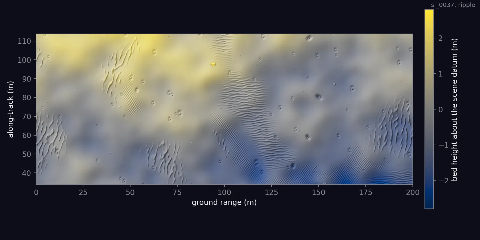
Shaded height map of the rippled seafloor with a colour bar in metres
The height mapthe 16-bit DEM decoded to metres with the scale in its own metadata, cropped to the imaged 80 m and shaded
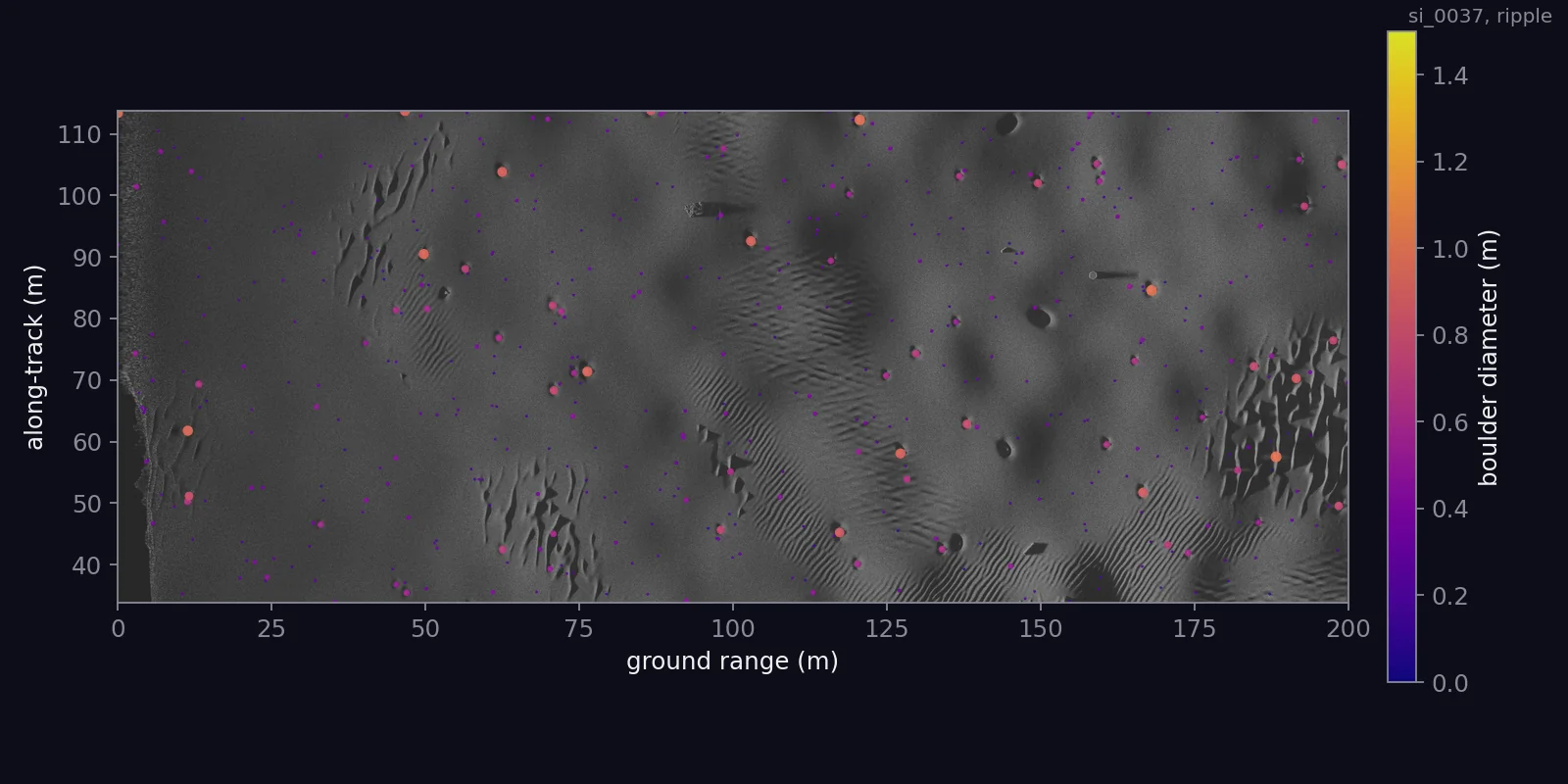
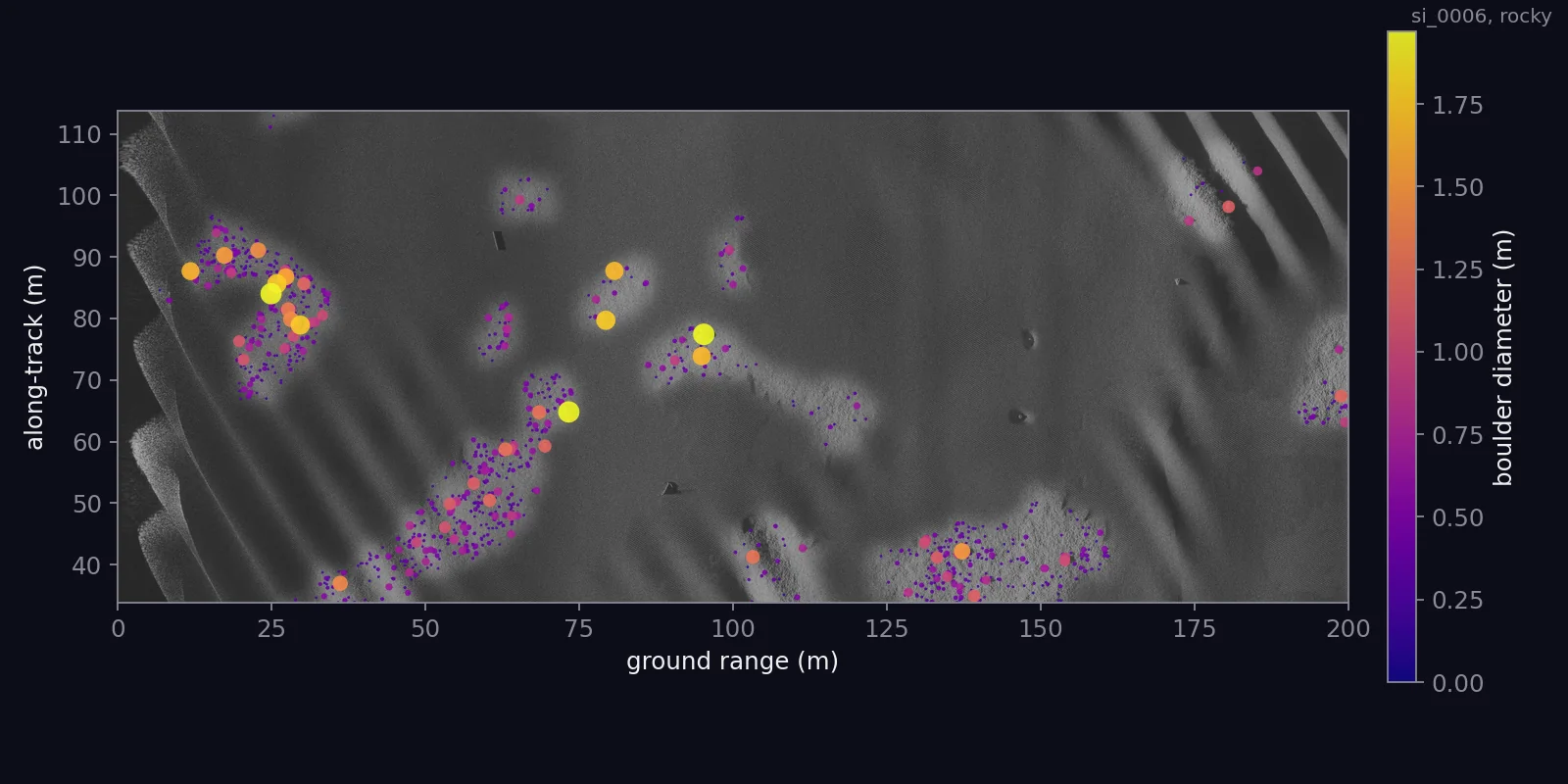
The swath in grey with each boulder of its rocks table marked by diameter
The boulder tableeach row of the rocks CSV in the imaged band, placed with the beamformer's mapping and coloured and sized by diameter

A rocky seafloor

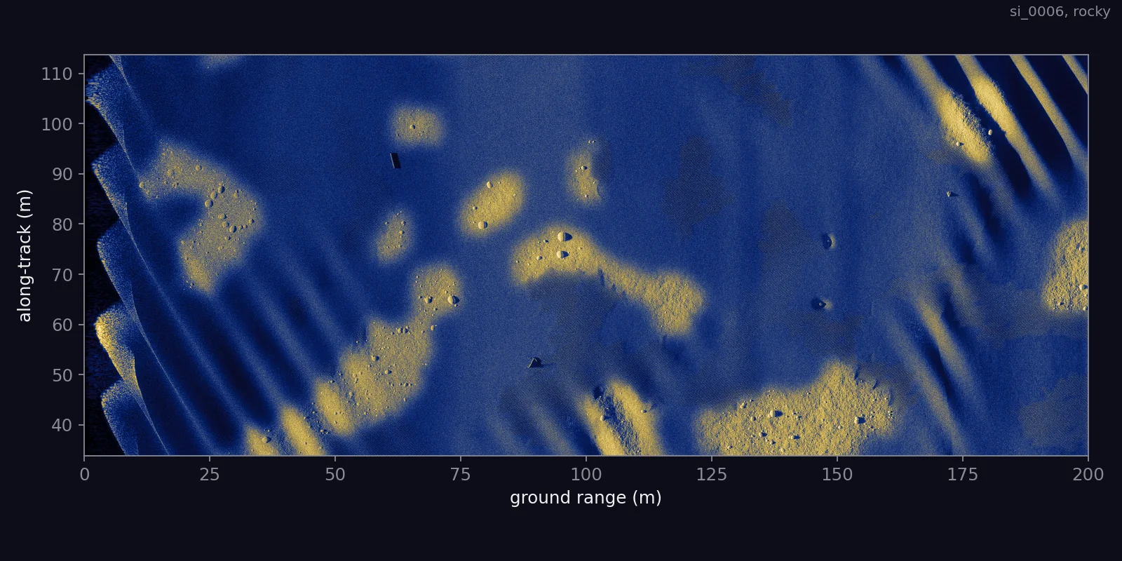
Whole v1.1 swath of a rocky seafloor with many boulders
The imagethe whole swath, reduced from 8000 by 3200 px
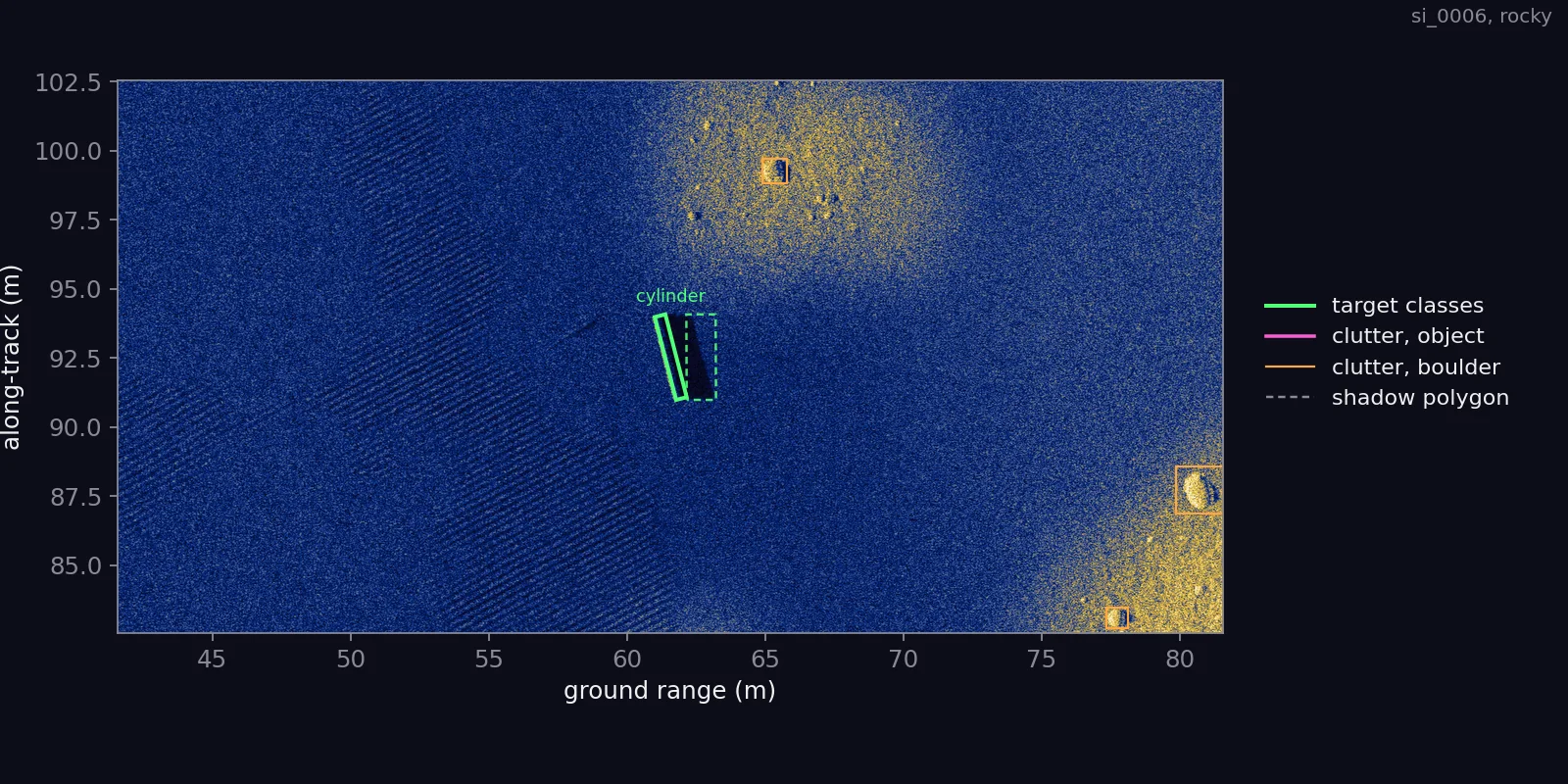
A 40 m by 20 m window of the rocky swath with target, clutter and boulder polygons drawn
A window, labelled40 m by 20 m at full resolution, with the same colours as above; boulder labels are drawn in orange
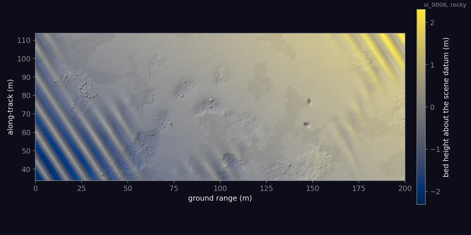
Shaded height map of the rocky seafloor with a colour bar in metres
The height mapthe DEM over the imaged band, height about the scene datum in metres
The rocky swath in grey with its boulders marked by diameter
The boulder tablethe rocks CSV in the imaged band; only boulders of 0.75 m and larger become clutter annotations

A sediment patchwork

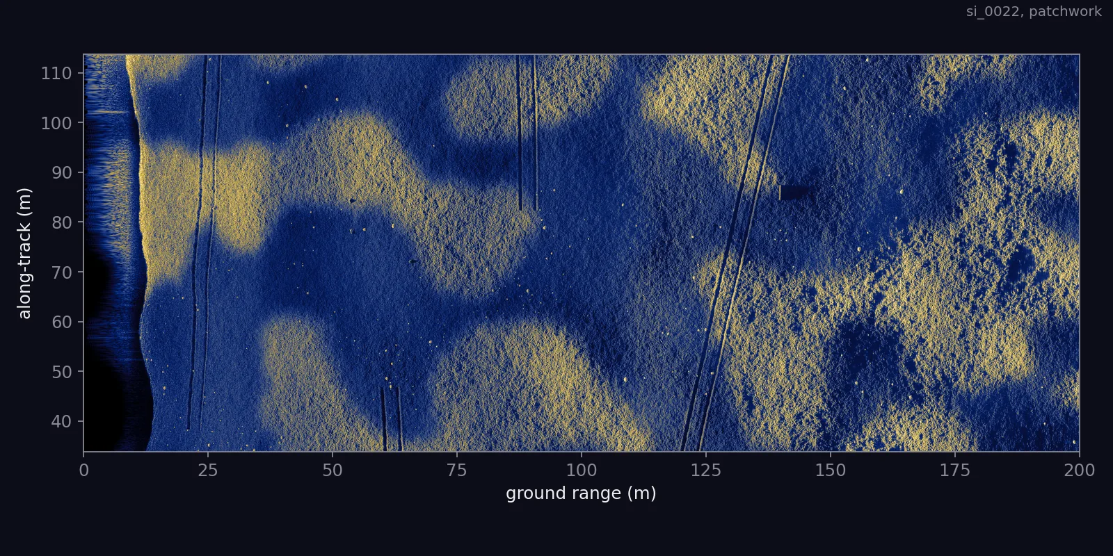
Whole v1.1 swath of a patchwork of sediment types
The imagethe whole swath, reduced from 8000 by 3200 px
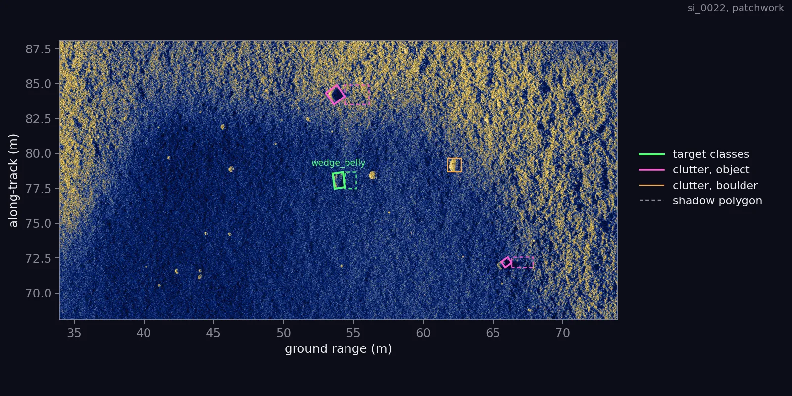
A 40 m by 20 m window of the patchwork swath with its label polygons drawn
A window, labelled40 m by 20 m at full resolution, with the same colours as above
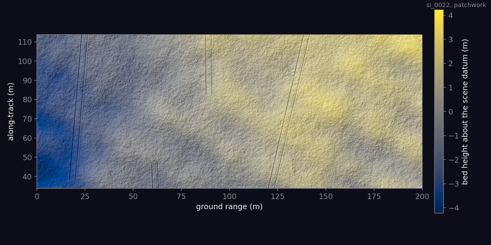
Shaded height map of the patchwork seafloor with a colour bar in metres
The height mapbathymetry, tilt and bedforms together, height about the scene datum in metres
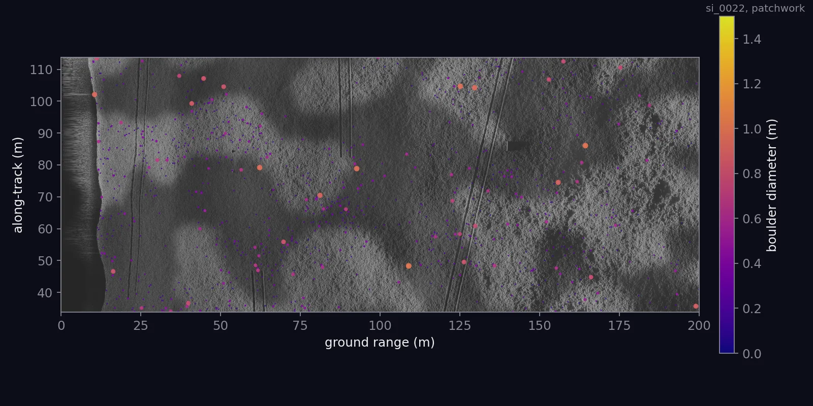
The patchwork swath in grey with its boulders marked by diameter
The boulder tablethe rocks CSV in the imaged band, coloured and sized by diameter

Georeference

A track that starts at latitude 0, longitude 0 and runs north.

Each image is georeferenced so that GIS tools open it at a consistent scale and orientation. The frame is a transverse Mercator on the prime meridian at the equator, on the WGS 84 datum, with unit scale and no false origin:

+proj=tmerc +lat_0=0 +lon_0=0 +k=1 +x_0=0 +y_0=0 +datum=WGS84 +units=m

The platform track starts at (0, 0) and runs north, so northing is metres along track and easting is metres of ground range to starboard. The location is a convention for the tools, not a place on the seafloor; every swath sits at the same nominal origin.

Limits

What it is not.

Back to all datasets, or read how the labels are emitted.