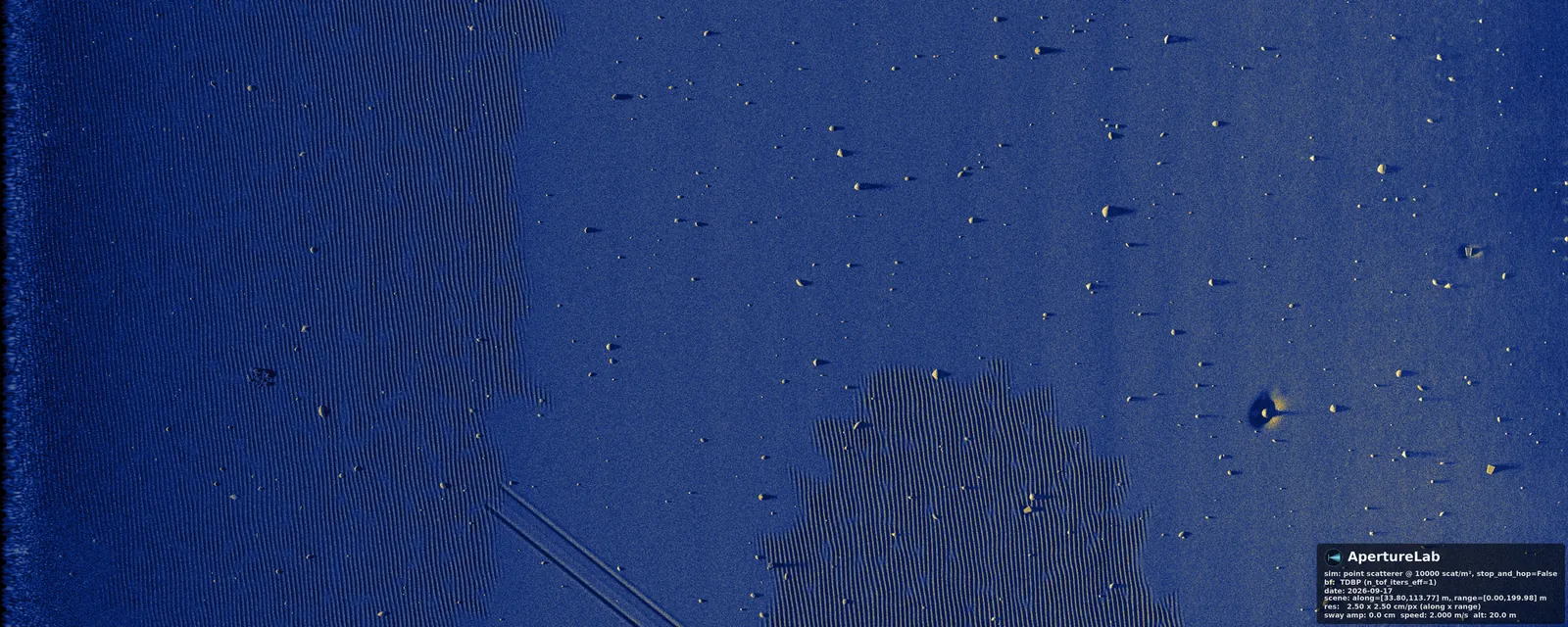
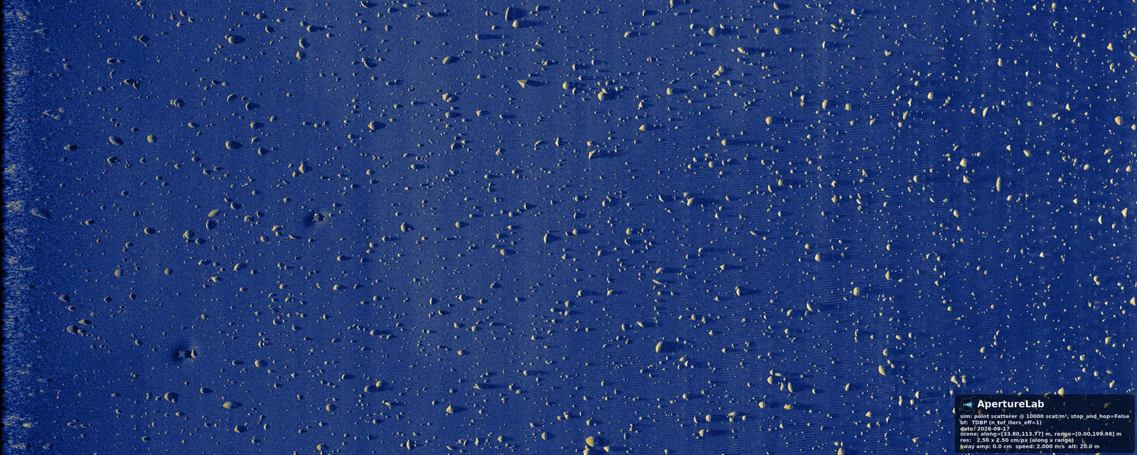
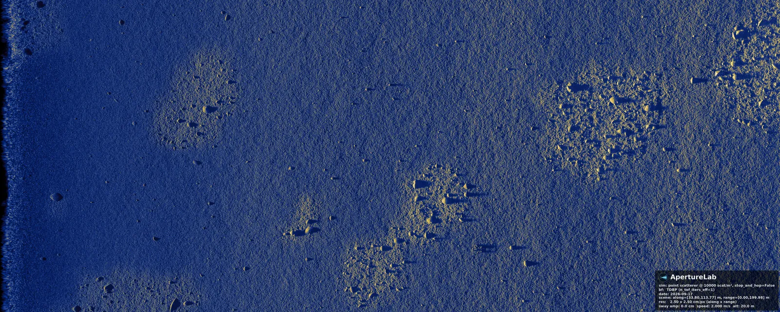
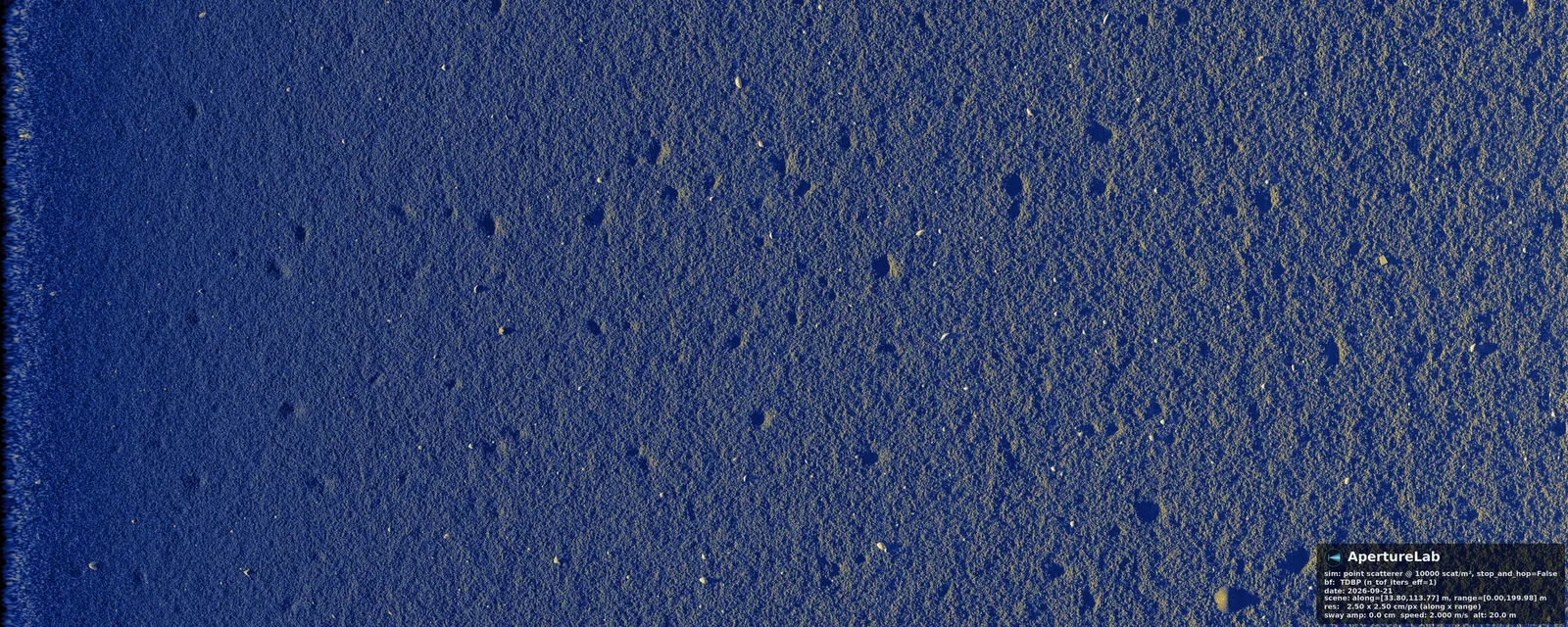
One thousand labeled sonar swaths, free to download.

Labeled sonar imagery has never existed at the scale modern vision models need. Collecting it takes ships, dive operations and restricted access, and labeling it takes a trained analyst for every object in every scene. The ApertureLab Synthetic SAS Dataset, version 1.0, is a first answer to that gap: one thousand synthetic aperture sonar swaths from a HISAS-class sonar, simulated end to end with ApertureLab, each with exact COCO labels and the scene file that produced it. It is on Hugging Face, free for research and commercial use under a license that names a few excluded organisations.

This page describes version 1.0 as published on 21 September 2026. Version 1.1, which re-issues the same footprint with terrain-aware labels, georeferenced images and metres of seafloor relief, and labels four target shapes and 23 kinds of clutter as 27 categories without the image-sized seafloor boxes, is being regenerated; see its page, or all datasets side by side.

By the numbers

What is in it, counted from the files.

Every figure below is read from manifest.csv, objects.csv and coco_all.json in the published dataset by tools/build_dataset_page.py, so every figure can be recomputed from the download.

4.7 nmi²

of labeled seafloor in total (16 km²): 1000 swaths of 200 m range by 80 m along track at 2.5 cm pixels

coco_all.json: range_extent_m, along_extent_m, pixel_size_m

1000

images, 8000 by 3200 px, TIFF LZW; 800 train, 100 validation, 100 test

manifest.csv: split

2000

labeled targets: 1000 truncated cones and 1000 wedges, one to six per scene, 150 scenes with none

objects.csv: role = target

2479

labeled clutter objects across 22 classes: ten meshes and twelve parametric shapes

objects.csv: role = clutter

seafloor families: uniform 331, patchwork 288, ripple 219, rocky 153, and 9 pockmarked scenes held out in the test split

manifest.csv: family

5503

COCO polygon annotations over 27 categories, including trawl scars and pockmarks as seafloor features

coco_all.json: annotations, categories

Targets sit on sand (815), gravel (445), mud (300), silt (283) and rock (157), with substrate-dependent burial: the median target is buried to about a tenth of its height, 249 are buried past a third, and the deepest to 0.70 of its height, in mud. Grazing angles run from 6 to 53 degrees across the swath. Clutter comes in three tiers per scene, from none to eight objects, and includes tires, oil drums, kegs, anchors, fish traps, ladders, pallets, propellers, debris and rock piles, plus pyramids, cones, frustums, domes, drums, slabs, hexagonal prisms, capsules, crosses, random polyhedra, sediment mounds and tori.

Labels per class

Every COCO category, counted by split.

The 1000 images split 800 train, 100 validation and 100 test. The table counts labeled instances, one row per COCO category, read from coco_all.json with each image's split taken from manifest.csv. In v1.0 every clutter shape is its own category, so clutter appears as 22 rows with a subtotal. The total of 5503 is more than the 2000 targets and 2479 clutter objects above because it also counts the 772 boulders labeled rock, 243 trawl scars and 9 pockmarks. Pockmarks appear only in the test split, where the pockmarked seafloor family is held out.

class	train	val	test	total
Targets
`truncated_cone`	809	92	99	1,000
`wedge`	776	105	119	1,000
targets, 2 classes	1,585	197	218	2,000
Clutter
`dome`	135	20	23	178
`hexprism`	123	16	19	158
`torus`	122	17	15	154
`mound`	110	16	22	148
`polyhedron`	118	12	18	148
`cross`	112	14	17	143
`capsule`	116	18	8	142
`drum`	111	17	12	140
`slab`	108	14	16	138
`pyramid`	101	15	20	136
`cone`	104	14	17	135
`frustum`	97	11	13	121
`ladder`	68	8	9	85
`ship_propeller`	69	6	6	81
`tire`	69	9	2	80
`keg`	58	7	14	79
`europalette`	62	8	3	73
`fish_trap_square`	61	7	4	72
`debris1`	55	7	8	70
`sunken_anchor`	54	7	8	69
`barrel_oil`	49	6	10	65
`rock_pile`	52	5	7	64
clutter, 22 classes	1,954	254	271	2,479
Other labeled objects
`rock`	622	72	78	772
`trawl_scar`	206	19	18	243
other labeled objects, 2 classes	828	91	96	1,015
Seafloor features
`pockmark`	0	0	9	9
all labels, 27 classes	4,367	542	594	5,503

Browse it

Eight swaths, one per seafloor family and clutter tier.

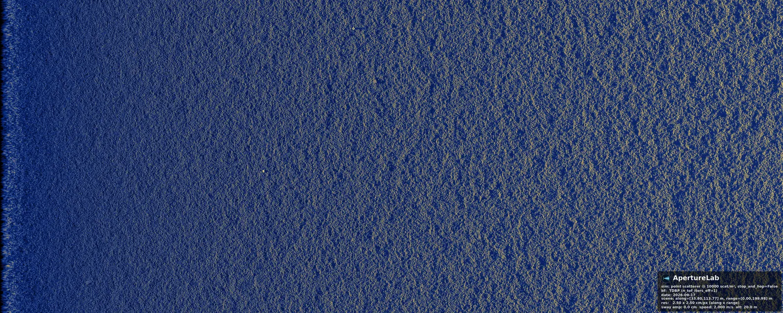
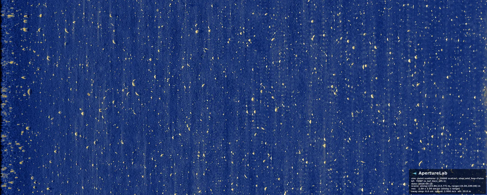
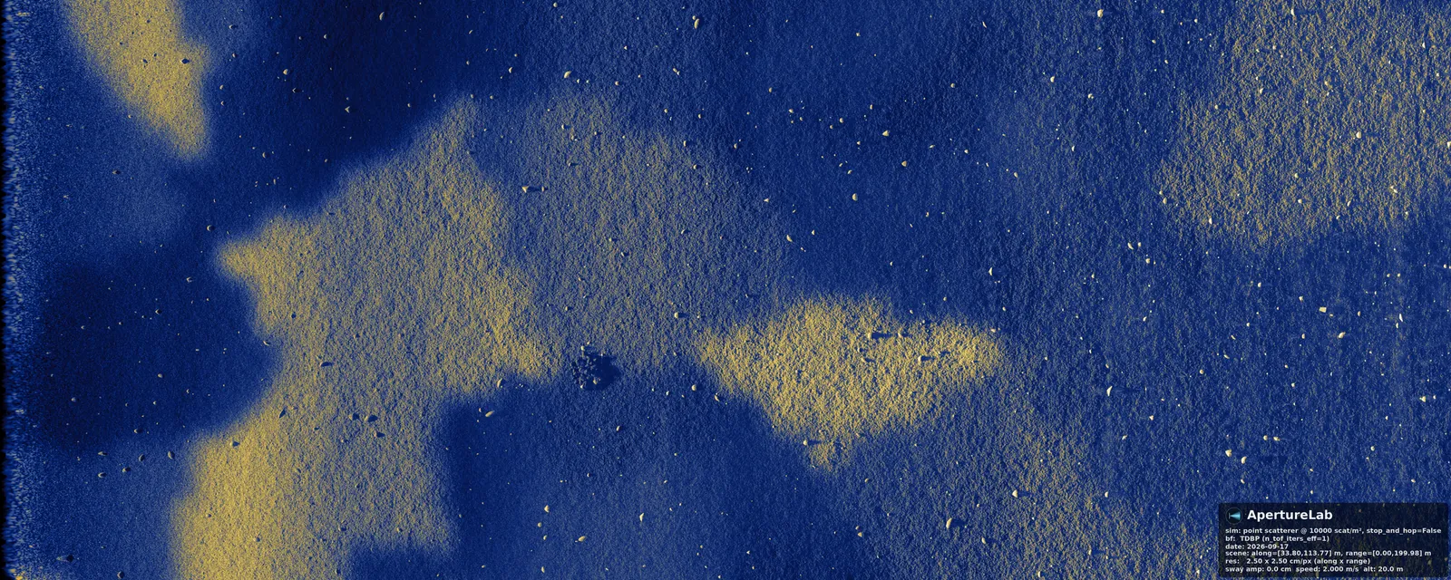
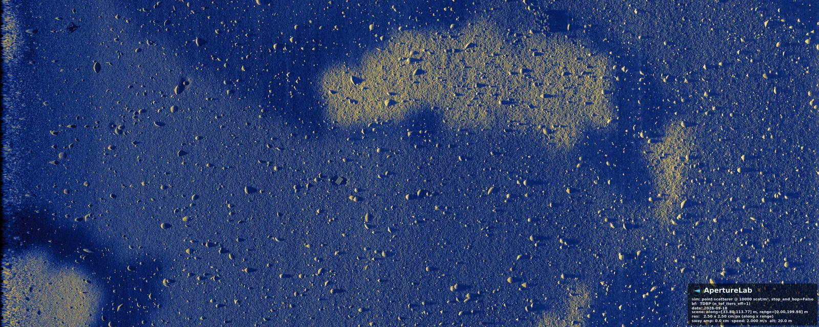
Each image below is a whole swath, reduced to fit; the sonar track runs up the left edge and range increases to the right. Click any one to open it larger. At this scale a target is a few pixels wide; the chips further down show them at native resolution.

Uniform silt seafloor swath with no clutter tier and five targets

Uniform seafloor, no clutter tier: one cone, four wedges, one stray object.

Uniform seafloor swath with the dense clutter tier

Uniform seafloor, dense clutter tier: two cones, three wedges, five clutter objects.

Patchwork seafloor swath with two wedges

Patchwork of sediment types, light clutter: two wedges.

Patchwork seafloor swath with the dense clutter tier

Patchwork, dense clutter: three cones, one wedge, eight clutter objects.

Rippled sand swath with trawl scars and rock clutter

Ripple fields on sand with trawl scars: two cones, three wedges, four clutter objects.

Rippled seafloor swath with the dense clutter tier

Ripple fields, dense clutter: two cones, one wedge, four clutter objects.

Rocky ground, light clutter: two cones, one wedge.

Pockmarked seafloor swath from the held-out test family

Pockmarked seafloor, the family that appears only in the test split: one cone, two wedges.

A known defect in v1.0: the scene runner burned its information box into the lower-right corner of every image (about 32 m by 11 m of the far range at the start of the track). It is documented in the dataset card and the labels are correct underneath it.

At native scale

The targets, with the label that ships with them.

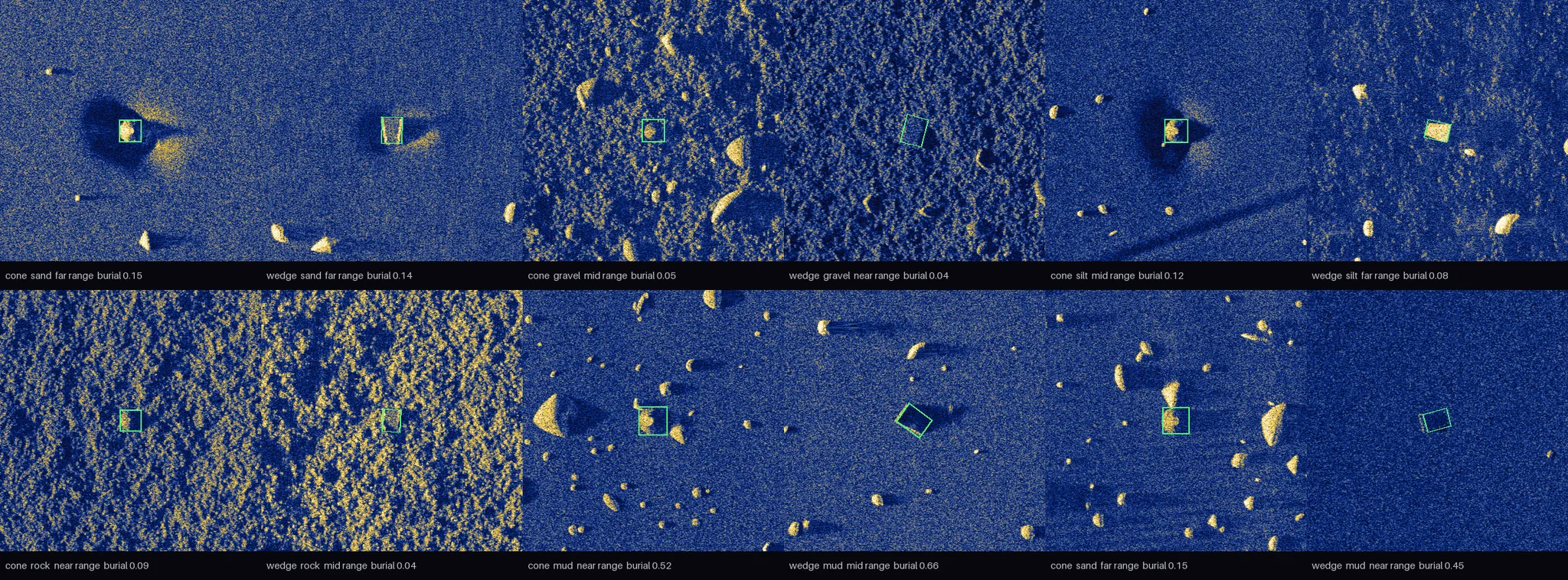
Twelve 10 m chips at the dataset's own resolution, one target each, with its COCO polygon drawn in green. The polygon is the object's footprint and heading, projected into the image from the scene file. It does not follow the bright return or the shadow, which is why a polygon can sit at the edge of a highlight rather than around it; that is the correct position of the object. The sand, gravel, silt and rock chips are exposed targets; the two mud chips are buried past half their height, which is why they show less highlight and less shadow.

Twelve sonar chips of truncated cones and wedges on sand, gravel, silt, rock and mud, each with a green polygon marking the labeled object footprint — Cone and wedge on each substrate, near and far range, exposed and buried. Each chip is 400 by 400 pixels, 10 m on a side. The caption under each chip is read from the annotation's attributes.

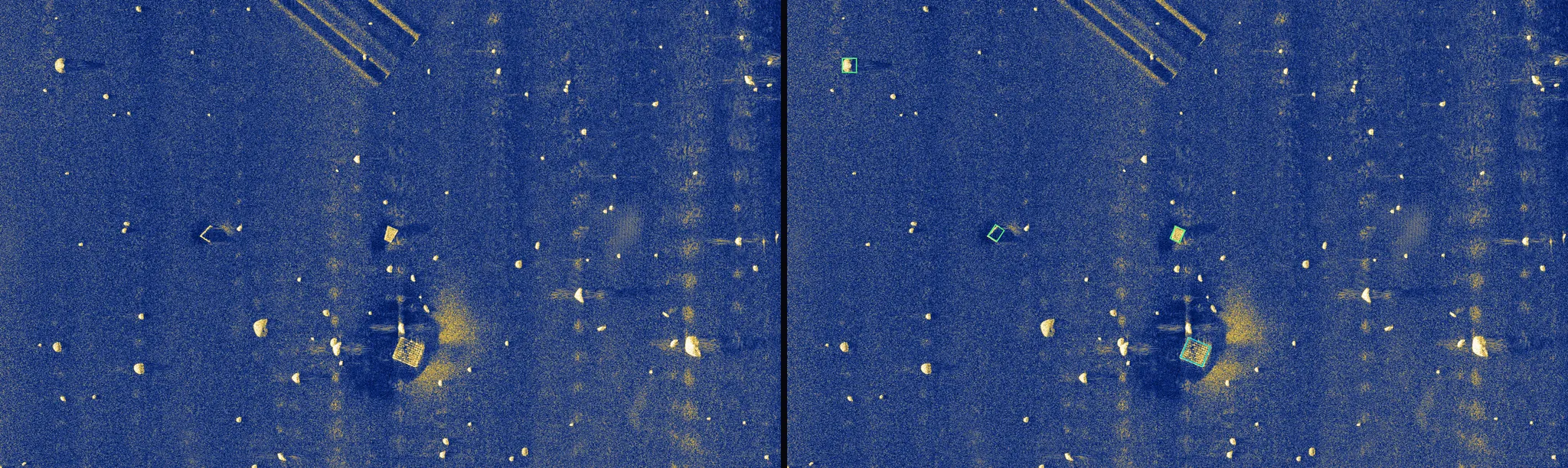
A 50 m by 30 m crop of a seafloor shown twice, the second copy with green target polygons and cyan clutter polygons drawn — One 50 m by 30 m crop, clean and then labeled. Green: the two target classes. Cyan: clutter, which carries its own class in the COCO file and a `role: clutter` attribute, so a detector can be trained on the target classes alone or on every class.

How it was made

From a scene file to a sonar image.

A generator draws each scene from a master seed: a seafloor family, a substrate, a ripple wavelength and direction where there are ripples, a clutter tier, and the targets, which are allocated so the set holds exactly a thousand of each class. The scene is written as YAML. That file is the whole specification, and it ships in the dataset, so a scene can be edited and rendered again.

The simulator builds the heightfield from the file, seats every object into the local bed with substrate-coupled burial and scour, and flies the sonar along a straight line at 20 m altitude. The time-domain back-projection beamformer then forms the image. Each swath took about five minutes on one workstation GPU at ten thousand scatterers per square metre.

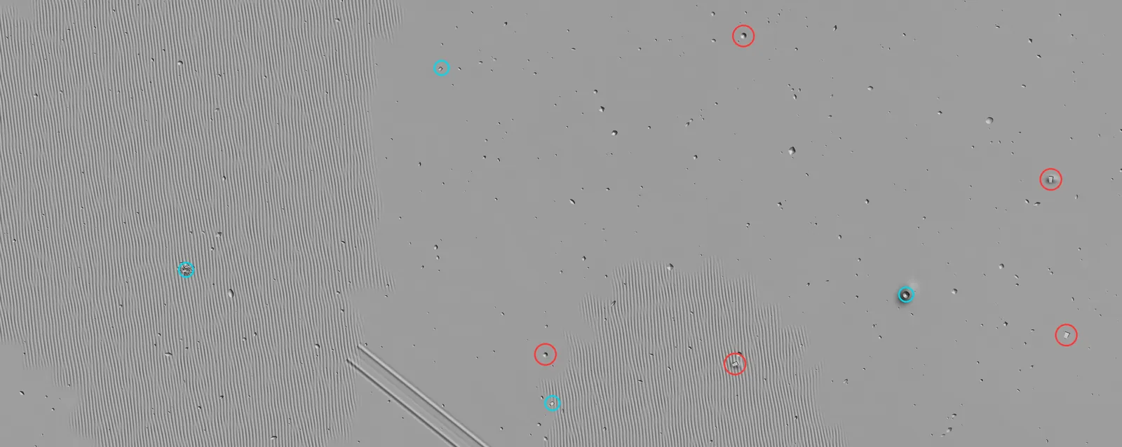
Grey heightfield of a rippled sand scene with trawl scars, red rings on the five targets and cyan rings on the clutter — The heightfield the simulator built for scene si_0008, cropped to the 80 m the image covers: ripple patches, two trawl scars, rocks. Red rings: targets. Cyan: clutter.

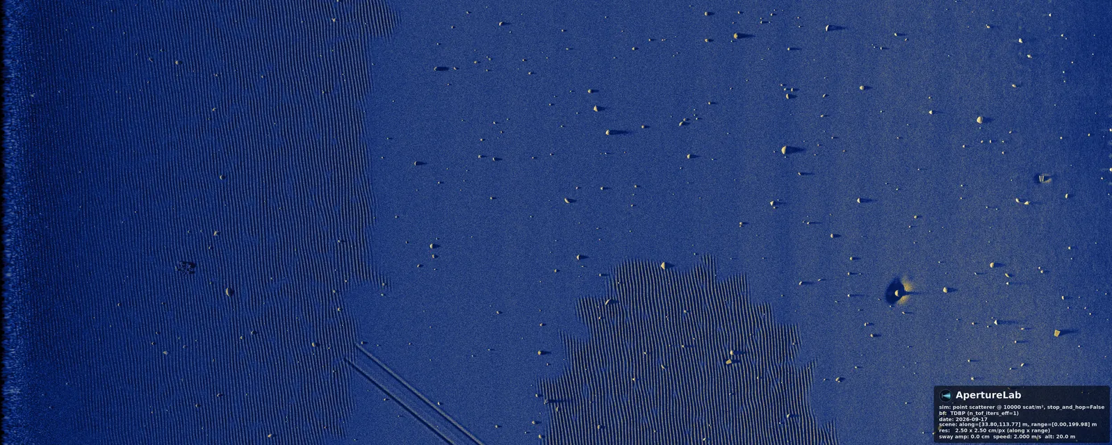
The sonar image formed from the same rippled scene — The same 80 m as the sonar sees it.

An excerpt of that scene's file, with the 40 by 50 zone grid and the other objects elided:

name: si_0008
description: 'sample_images_1000 #8: ripple (sand, clutter L1), 2 cones + 3 wedges, 4 clutter.'
bottom:
  default_type: sand_r0
  seed: 373871
  zone_grid: ...            # 40 x 50 cells of 4 m, one substrate token each
objects:
- kind: wedge
  name: wedge_0008_0
  x: 53.822
  y: 190.083
  ts_db: -13.37
  scale: 1.091
  seed: 648360
  heading_deg: 21.0
  scour: {enabled: false, sediment_type: sand, burial_fraction: 0.283}
  annotation: {class: wedge, range_band: far, substrate: sand, burial_fraction: 0.283, grazing_deg: 6.01}
- ...
motion: {kind: straight_line, speed: 2.0, altitude: 20.0, n_pings: 246, ping_rate: 3.33}
sonar: {fc: 100000.0, bandwidth: 30000.0, n_channels: 32, channel_spacing: 0.04, sonar_side: starboard}
beamform: {pixel_spacing: 0.025, along_track_length: 80.0, range_max: 200.0}

The sonar is the HISAS 1030 preset: 100 kHz centre frequency, 30 kHz of bandwidth, 32 channels at 40 mm; consecutive pings share two phase centres, which is the overlap a survey sonar uses in practice. The generator and its design document are in the ApertureLab repository under simulator/scenes/sample_images/.

Get it

On Hugging Face, with the license beside the images.

Repository: huggingface.co/datasets/idg101/Aperture_Lab_Synthetic_Aperture_Sonar_v1. The images total about 40 GB.

images/si_XXXX_*_tdbp_drc.tif: the image, 8000 by 3200 px, TIFF LZW, along-track up, range right.
images/si_XXXX_*_tdbp_coco.json: that image's COCO polygons, with world extents and pixel size on the image record and class, substrate, burial, range band and grazing angle on each annotation.
coco_all.json: the same, merged over the whole set.
manifest.csv: one row per scene, with split, seafloor family, clutter tier and object counts.
objects.csv: one row per object, targets and clutter, with position, heading, size, substrate and burial.
scenes/si_XXXX.yaml: the scene file, editable and re-runnable in ApertureLab.

What it is not, so that the decision to download is an informed one:

It is simulated. The physics is validated against published scattering models and the textbook point-spread function, but none of it is field data.
One sonar, one straight track, no navigation error. There is no motion-error augmentation and no second geometry in this version.
Two target classes. Everything else that is labeled is clutter.
An information box is burned into the lower-right corner of every image, as described above.
The heightfields are not included; the scene files regenerate them.

The license (ALSD-1.0, in LICENSE.md) grants use, redistribution, derivative works and model training for any purpose, with attribution, on the condition that redistributions carry the same terms. It withholds all rights from four organisations named in the license. If you use the dataset, please cite:

Gerg, I. (2026). ApertureLab Synthetic SAS Dataset, version 1.0: 1000 HISAS-class swaths with cone and wedge targets. https://huggingface.co/datasets/idg101/Aperture_Lab_Synthetic_Aperture_Sonar_v1

Next: version 1.1, all datasets, or how the labels are emitted.