DRAFT · this page is currently under construction.

Motion estimation and image formation on independent stave data

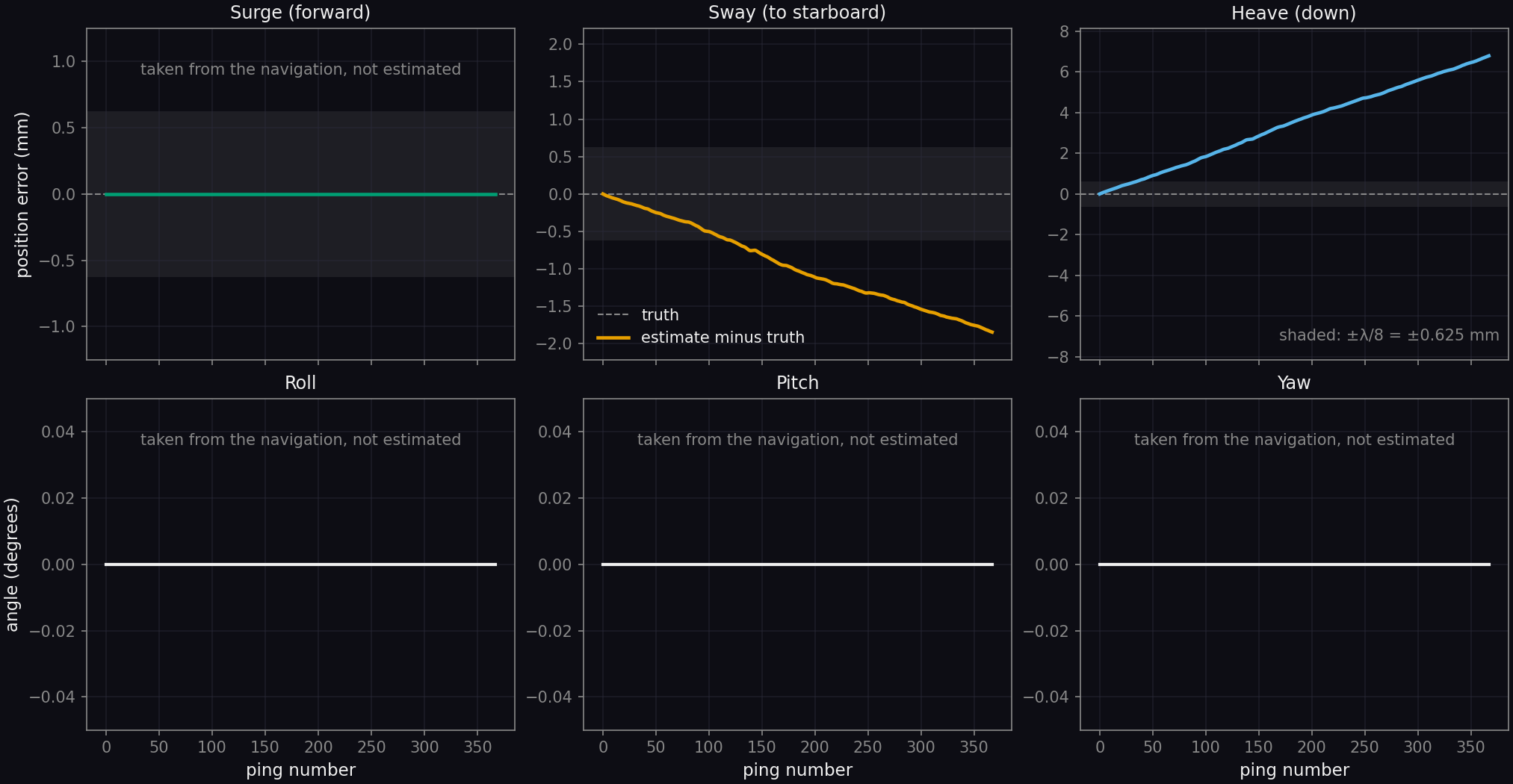
ApertureLab's motion estimation and back-projection were applied to stave data that ApertureLab did not generate: the University of Bath's simulated interferometric synthetic aperture sonar (InSAS) record of the SS Thistlegorm wreck [1, 2]. With sway and heave estimated from the echoes alone, the estimated track ends 1.8 mm to port of the true track and 6.8 mm below it after 200 m, and the image formed with it has a magnitude correlation of 0.9995 with the image formed with the true track. The vehicle in this record flies a straight line, so the result shows that the estimator reports no motion where there is none, in a scene where a wreck rising about 17 m from the seabed and its shadows fill much of the swath. The second part of the page applies the same estimator to a sonar simulated along a recorded vehicle track over a seabed with relief, and compares it with the navigation the vehicle's sensors report.

Data

The Bath simulated InSAS record

Thomas and Hunter simulated the record from a three-dimensional model of the wreck on a textured seafloor, a scene of 220 m by 135 m, with a point-based scattering model and ray-traced occlusion [1, 2]. The sonar is similar to the 300 kHz MUSCLE system of the NATO Centre for Maritime Research and Experimentation. The data are distributed under the Creative Commons Attribution 4.0 license. No noise and no motion were added to the record for this page.

Pings
The record holds 368 pings at an interval of 0.1 s along a straight track of 199.8 m, with roll, pitch and yaw of zero throughout.
Staves
Each ping holds 72 receiver channels, two rows of 36, of which one row is used on this page.
Signal
The center frequency is 300 kHz and the bandwidth 60 kHz, stored as complex baseband samples at 75 kHz after pulse compression and compensation for spherical spreading.
Range
Each channel holds 13,751 samples from 37.5 m to 175 m of slant range; the first seabed echo arrives at about 52 m.
Platform motion during an echo
The delays measured between shared phase centers show that the vehicle is stationary while each echo is received, so the data were processed without motion during the echo.
Sound speed
The sound speed is 1500 m/s, which gives a wavelength of 5 mm.

Array

Array geometry and ping overlap
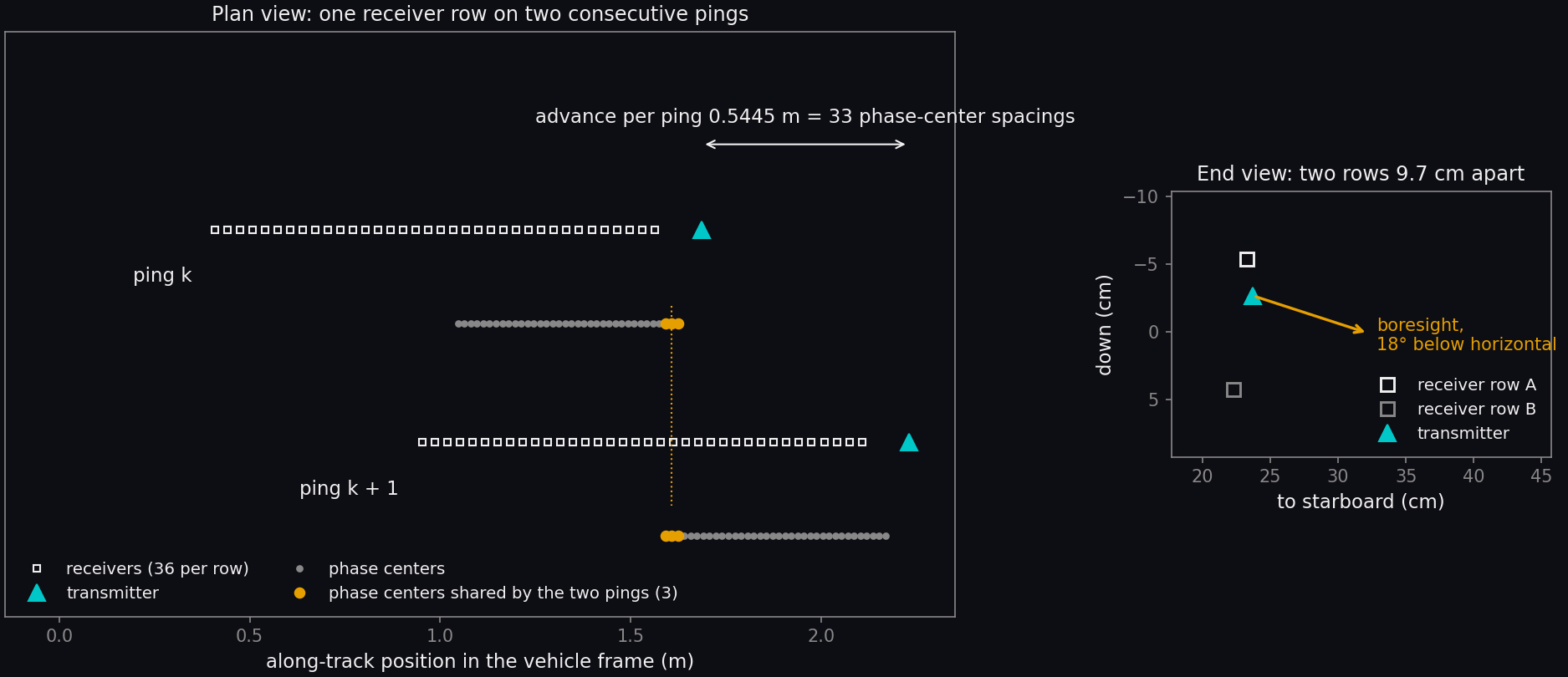
Two diagrams. The plan view shows one row of 36 receivers and a transmitter ahead of it for two consecutive pings, the second displaced forward by 0.5445 meters. Under each row is the line of phase centers; the last three of the first ping and the first three of the second are highlighted and aligned. The end view shows the transmitter and the two receiver rows 9.7 centimeters apart, with an arrow for the boresight pointing 18 degrees below horizontal to starboard.
The array as given in the dataset's metadata, in the vehicle frame. Left: one receiver row and the transmitter on two consecutive pings, with the phase centers (the midpoints of the transmitter and each receiver) drawn under them. Right: the two receiver rows and the transmitter seen from behind; the array looks to starboard.

The receivers are 33 mm apart, so the phase centers are 16.5 mm apart. The vehicle advances 0.5445 m between pings, which is 33 phase-center spacings on a row of 36, and three phase centers of each ping therefore coincide with three of the next. The echoes received at coincident phase centers differ only by what the vehicle did between the two pings, and the motion estimate is made from that difference. The transmitter measures 50 mm along the track and each receiver 33 mm.
Measurements

Correlation and time delay between shared phase centers

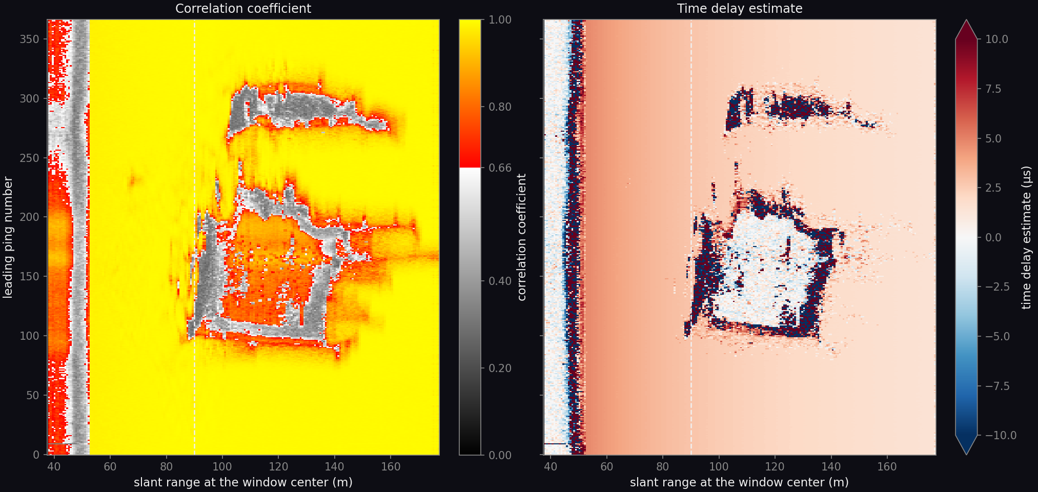
Two maps with leading ping number on the vertical axis and slant range from 37.5 to 178 meters on the horizontal axis. The correlation map is close to 1 over most of its area, with a band of low correlation before 52 meters and two irregular regions between about 90 and 155 meters outlined by low correlation. The time delay map falls smoothly from about 4 microseconds at 55 meters to about 1.5 microseconds at 170 meters, is near zero inside the same two regions, and is irregular along their edges and before 52 meters.
Correlation coefficient (left) and time delay estimate (right) of the echoes at shared phase centers, for each pair of consecutive pings and each range window of 128 samples. The correlation scale is gray below 0.66, the value under which a window is not used. The time delay scale is capped at ±10 µs. The dashed line is the far edge of the 20 m to 90 m range interval from which the motion is estimated.

Over the seabed the correlation coefficient is 0.99 and the time delay falls smoothly with range. On a straight track that delay is not zero: the two receivers of a shared phase center sit at different distances from the transmitter, which leaves a delay that depends on range alone. The motion model accounts for it, and over the seabed the measured and modeled delays agree to within 0.008 µs.

Two kinds of window hold no seabed echo: those before the first return at 52 m, and those in the two shadows of the wreck, which appear in the maps between 90 m and 155 m. The record's level there is about 40 dB below the seabed's, yet the channels still correlate above 0.66 in places, with a delay near zero that does not describe the vehicle. These windows are excluded by their level before the solve. The level the seabed returns at each range, and its spread, are read from the record itself. Of the 89,181 windows in the estimation interval, 26,934 were excluded as holding no seabed echo and 62,241 were used.

Result

Estimated motion against truth

Six plots against ping number from 0 to 367. Top row, position error in millimeters: surge is zero throughout and marked as taken from the navigation; sway falls in a straight line to minus 1.8 millimeters; heave rises in a straight line to plus 6.8 millimeters. A shaded band marks plus and minus 0.625 millimeters. Bottom row: roll, pitch and yaw in degrees, each zero throughout and marked as taken from the navigation.
Top: the estimated track minus the true track along the vehicle's axes, against ping number; the shaded band is one eighth of a wavelength, 0.625 mm, either side of zero. Bottom: the attitude of the vehicle. Sway and heave are estimated; surge, roll, pitch and yaw are taken from the navigation, which in this record is exact.

Sway and heave velocities are solved for all pings jointly by least squares on the time delay estimates, first with the delays from the correlation magnitude and then with the delays refined by the correlation phase, following [3]. The image formation page describes the chain this step belongs to.

The error in both axes grows in a straight line, which is a constant velocity bias: 0.05 mm/s in sway and 0.19 mm/s in heave, on a vehicle moving at 5.4 m/s. The position error passes one eighth of a wavelength after about 125 pings in sway and about 35 in heave. A constant velocity bias displaces the image and does not defocus it.

Images

Images formed with true and estimated navigation

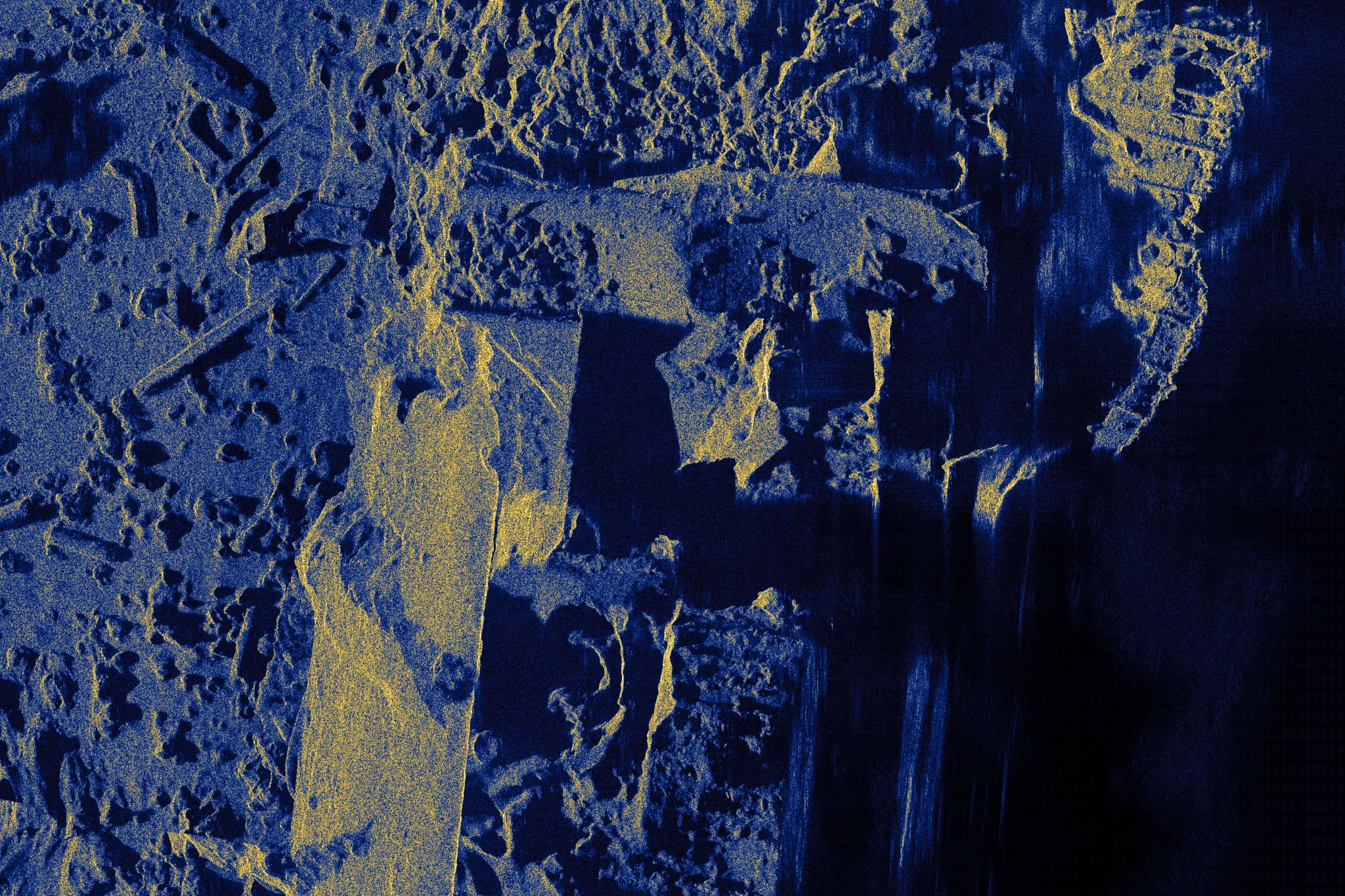
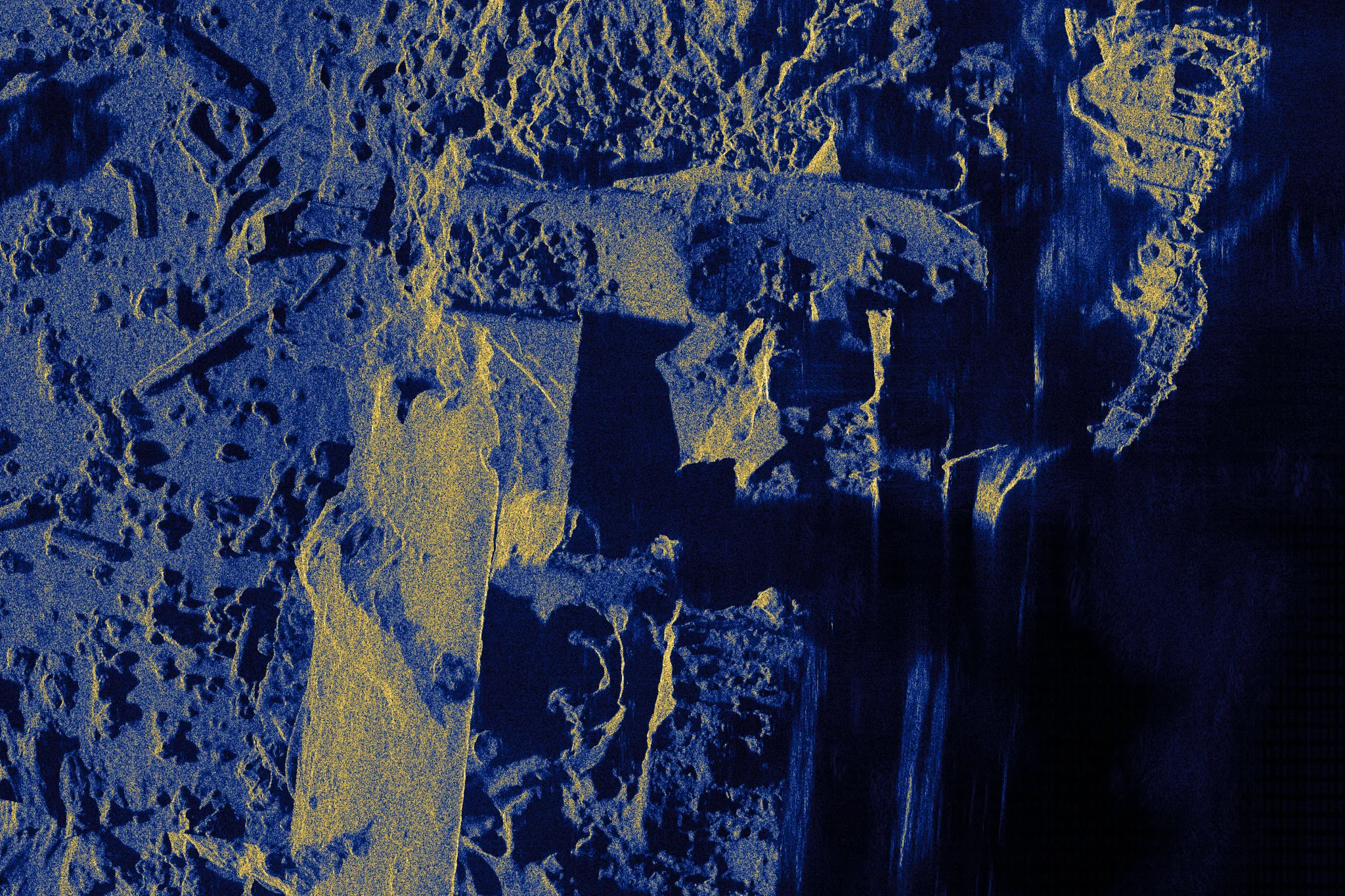
Synthetic aperture sonar image of part of the wreck at 2 centimeter pixels, formed with the true track: deck plating, structure and debris in fine detail, with acoustic shadows to the right. Estimated navigation True navigation
A 41 m by 27 m window on the wreck at the full 2 cm pixel spacing. The image formed with the estimated track is left of the divider and the image formed with the true track is right of it; the divider moves with the pointer or the arrow keys. Ground range increases to the right and the vehicle travels up the page. One range normalization and one tone map serve both images.
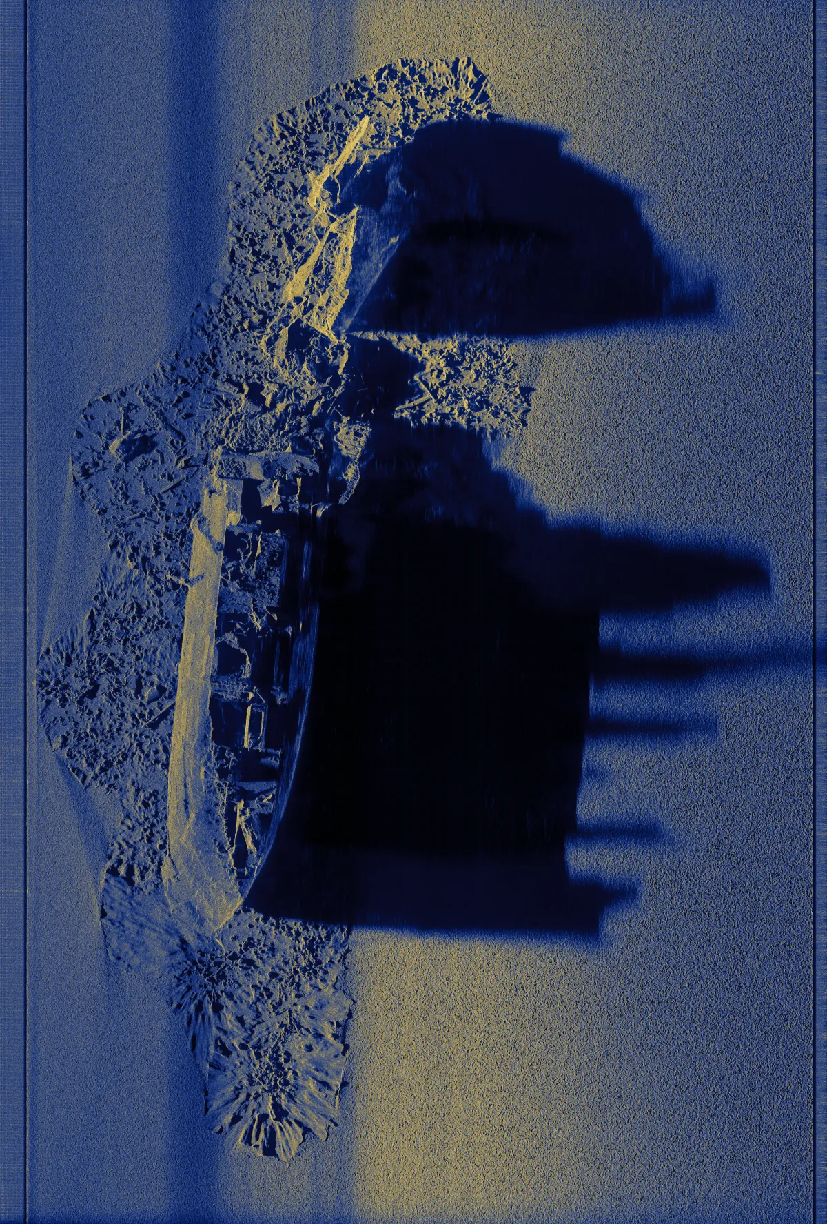
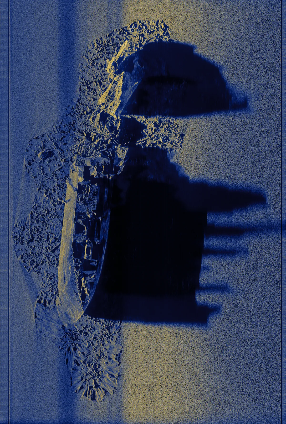
Synthetic aperture sonar image of the whole swath formed with the true track: the wreck lies along the track on the left half of the image with a debris field around it, and its shadows extend to the right. A band at mid range is brighter than the rest of the seabed. Estimated navigation True navigation
The whole swath, 135 m of ground range by 200 m of track, reduced from 6750 by 9992 pixels. Both images are focused on a horizontal plane 29.4 m below the track, the median depth of the seabed, so the wreck is displaced toward the track in proportion to its height. The brighter band at mid range comes from the range normalization of the display, which takes its level from all pings, including those in shadow at that range.

Motion

A simulated sonar on a recorded vehicle track

The Bath record holds no motion to recover. To measure the estimator where motion is present, a sonar of the same class was simulated in ApertureLab along a recorded vehicle track, together with the navigation its sensors would report. Three tracks are compared: the recorded track, which the simulation takes as true; the track dead reckoned from the sensors; and the track estimated from the echoes.

Scene
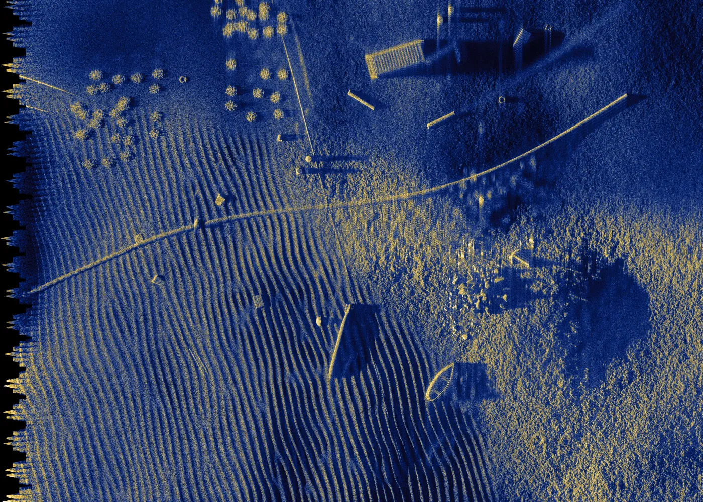
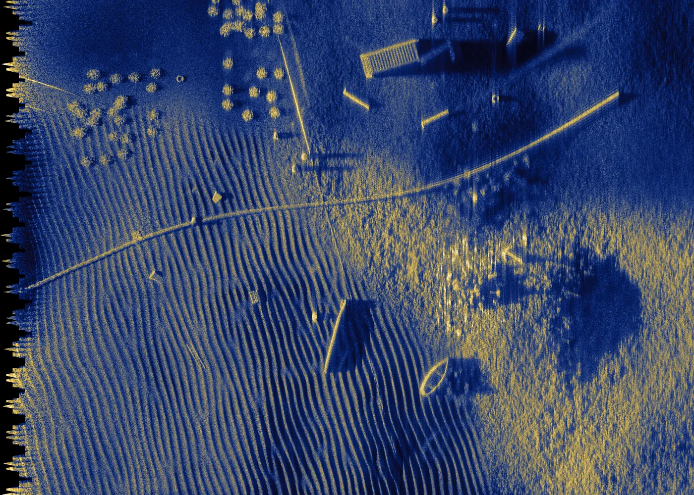
The scene is 70 m of ground range by 50 m of track: rippled sand, gravel and rock with a pipeline, a small boat and other objects. The seabed lies between 1.4 m below and 1.3 m above its mean height.
Sonar
The center frequency is 300 kHz and the bandwidth 60 kHz, with one row of 36 receivers 33.3 mm apart.
Track
The track holds 115 pings over 38 s and 60 m, at a mean speed of 1.57 m/s and 8 m above the mean seabed. The vehicle wanders 0.56 m from side to side with a period of 13 s and 0.26 m vertically, and it crabs by up to 5°. Yaw stays within 1.6°, pitch between 0.4° and 2.4° nose down, and roll changes by 0.3° from one ping to the next.
Ping timing and overlap
The interval between pings varies from 0.305 s to 0.360 s. The mean advance of 0.524 m is 31.4 phase-center spacings, which is not a whole number, so between four and five phase centers are shared and they do not coincide exactly.
Navigation sensors
A Doppler velocity log and an inertial unit are modeled with noise, bias and scale-factor errors, following the decomposition in [4]. The log's velocity noise is 4 mm/s per ping along and across the vehicle and 1.6 mm/s vertically; the inertial unit's attitude bias is 0.01° in roll and pitch and 0.02° in heading.
Inputs to the estimator
The estimator receives the reported attitude, altitude and forward speed, and returns surge, sway and heave velocities for every ping.

Measurements

Correlation and time delay with motion present

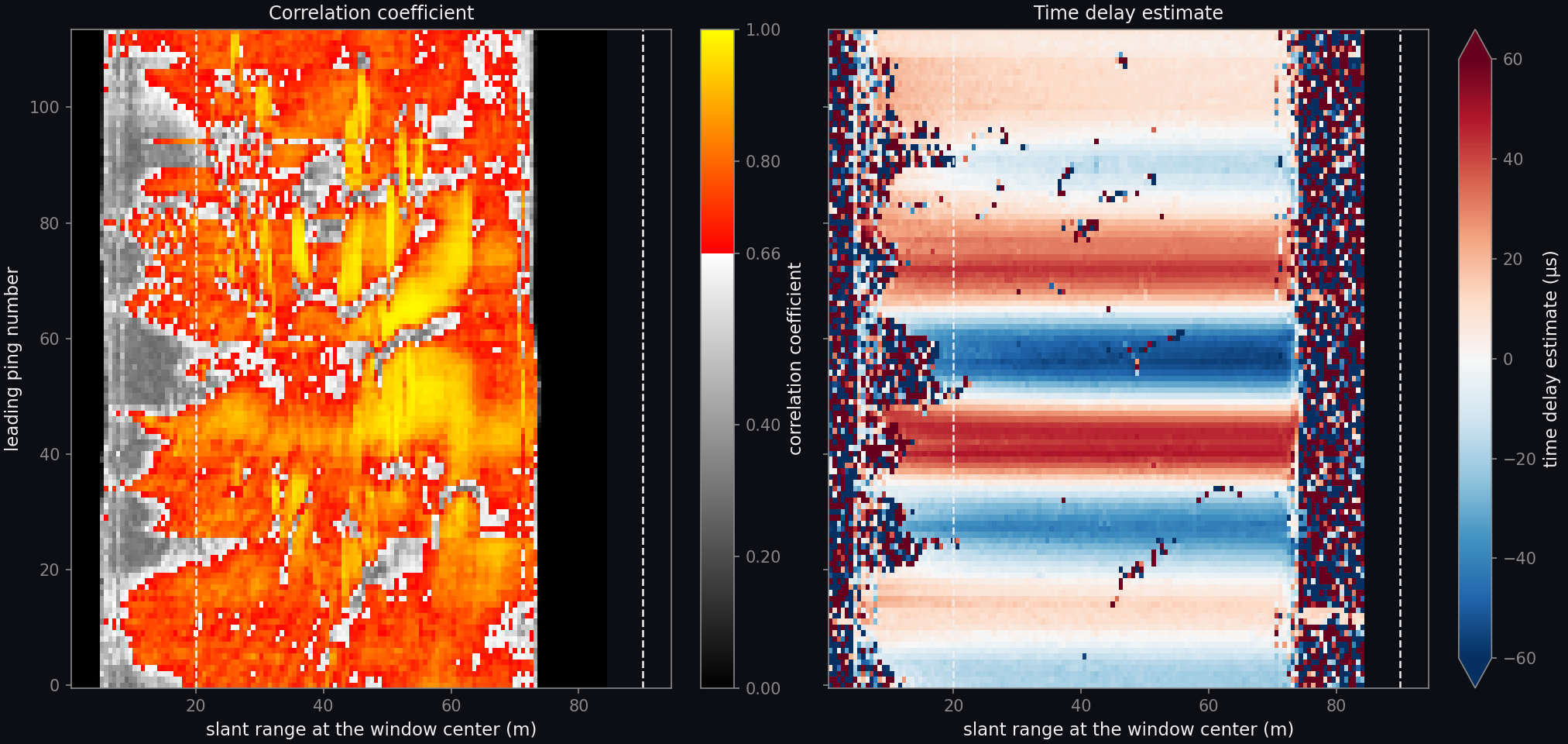
Two maps with leading ping number from 0 to 113 on the vertical axis and slant range from 0 to 90 meters on the horizontal axis. The correlation map is mostly between 0.66 and 1 from about 10 to 73 meters, with bands and patches of lower correlation, and is low inside 10 meters. The time delay map shows horizontal bands of alternating sign that follow the vehicle's sideways motion, reaching about 60 microseconds, nearly the same at every range between 10 and 73 meters, and is irregular outside that interval.
Correlation coefficient (left) and time delay estimate (right) of the echoes at shared phase centers, for each pair of consecutive pings and each range window. The correlation scale is gray below 0.66, the value under which a window is not used. The time delay scale is capped at ±60 µs. The dashed lines are the edges of the 20 m to 90 m range interval from which the motion is estimated; the record ends at 73 m.

The time delay follows the vehicle's sideways velocity from ping to ping and is nearly uniform across range, because the seabed is seen at shallow grazing angles. The median correlation coefficient in the estimation interval is 0.74, lower than on a track whose phase centers coincide, and 34,757 of its 52,100 windows are used.

Result

True, reported and estimated navigation

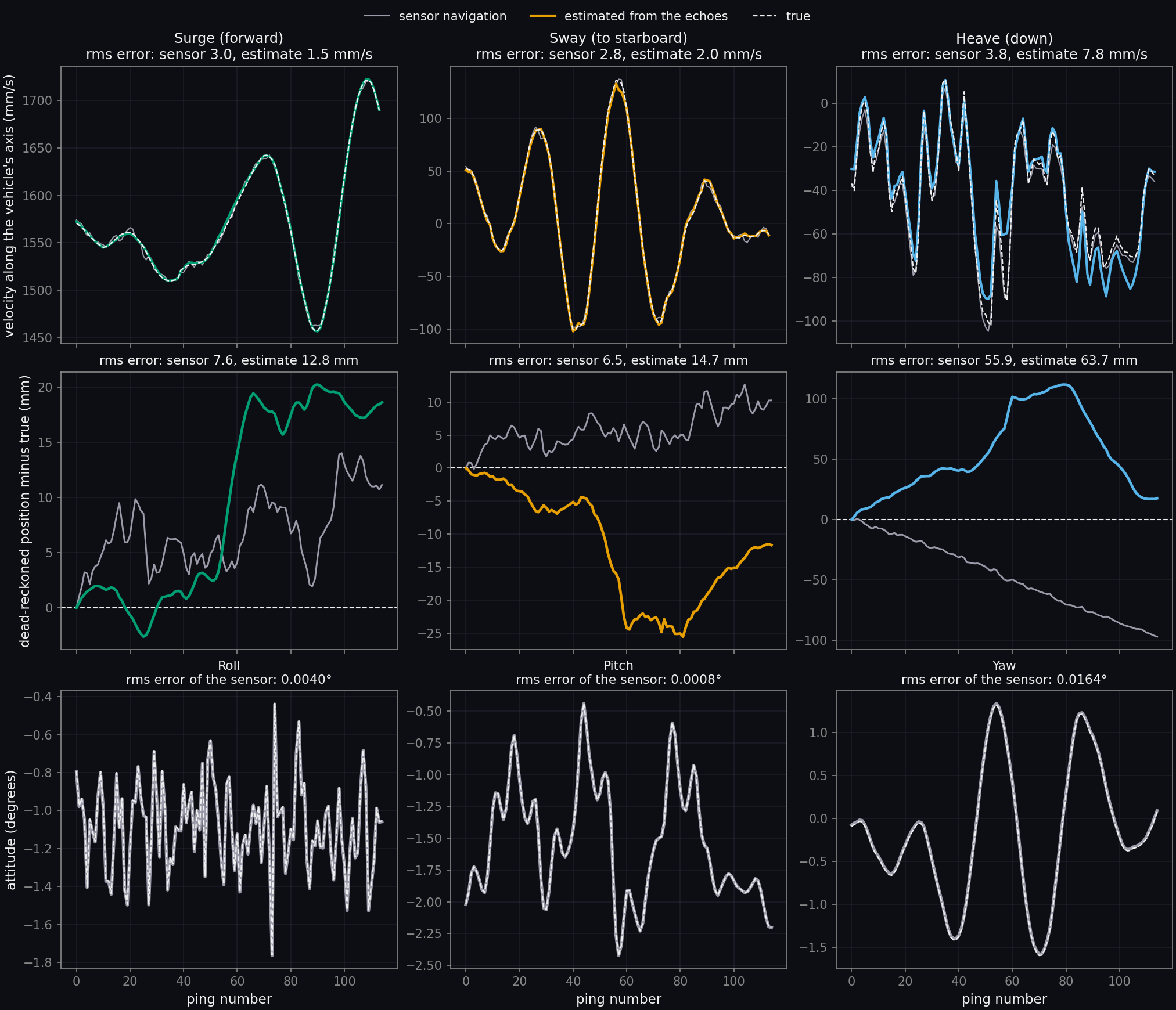
Nine plots against ping number from 0 to 114 in three rows. Top row, velocity along the vehicle's axes in millimeters per second: surge between 1460 and 1720, sway between minus 100 and plus 135, heave between minus 105 and plus 10; in each the sensor navigation and the estimate lie close to the dashed true curve, the estimate departing from it most in heave. Middle row, dead-reckoned position minus true in millimeters: the sensor navigation is an irregular line and the estimate a smoother one; in heave the estimate rises to 110 millimeters and returns to 18, while the sensor navigation falls steadily to minus 97. Bottom row, attitude in degrees: roll jitters between minus 1.8 and minus 0.4 from ping to ping, pitch varies between minus 2.4 and minus 0.4, and yaw swings smoothly between minus 1.6 and plus 1.3; the sensor and true curves coincide.
Top: the vehicle's velocity along its own axes as it truly was (dashed), from the track dead reckoned from the sensors (gray) and as estimated from the echoes (color). Middle: the position error each accumulates when dead reckoned from the first ping, along the same axes. Bottom: roll, pitch and yaw, true and as reported by the inertial unit; the estimator takes the attitude from the inertial unit and does not estimate it. The titles give the root-mean-square errors.

The root-mean-square velocity error of the estimate is 1.5 mm/s in surge, 2.0 mm/s in sway and 7.8 mm/s in heave, against 3.0, 2.8 and 3.8 mm/s for the sensor navigation. The two errors differ in character: the sensor error changes from one ping to the next, while the error of the estimate varies more slowly. Focus depends on the error across one synthetic aperture. At 45 m of range the sensor navigation leaves a phase error of 2.6 rad across the aperture once its mean and slope are removed, and the estimate leaves 1.0 rad.

Dead reckoned over the whole record, the estimate lies further from the true track than the sensor navigation does: 12.8 mm against 7.6 mm in surge, 14.7 mm against 6.5 mm in sway and 63.7 mm against 55.9 mm in heave. A slowly varying position error displaces the image and does not defocus it. The heave error of the estimate is attributed to the motion model, which assumes a horizontal seabed where this one varies by 2.7 m.

Images

Images formed with reported and estimated navigation

Synthetic aperture sonar image at 2 centimeter pixels formed with the estimated navigation: sand ripples, a curved pipeline, a small boat, a field of rocks and several smaller objects, each with a sharp outline and an acoustic shadow. Sensor navigation Estimated navigation
A 41 m by 27 m window at the full 2 cm pixel spacing, from 29 m of ground range outward. The image formed with the track dead reckoned from the sensors is left of the divider and the image formed with the estimated track is right of it; the divider moves with the pointer or the arrow keys. Ground range increases to the right and the vehicle travels up the page. One range normalization and one tone map serve both images.
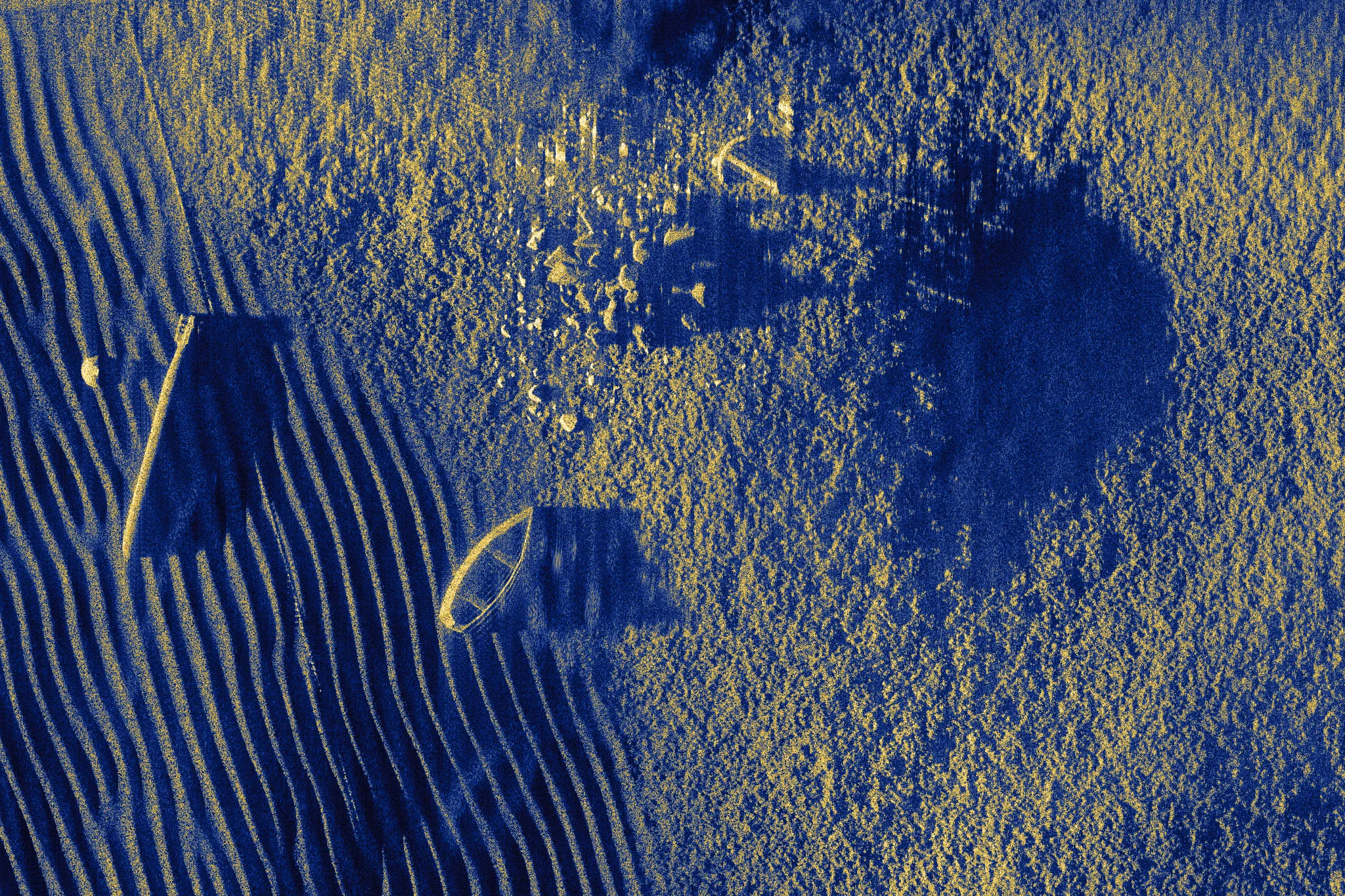
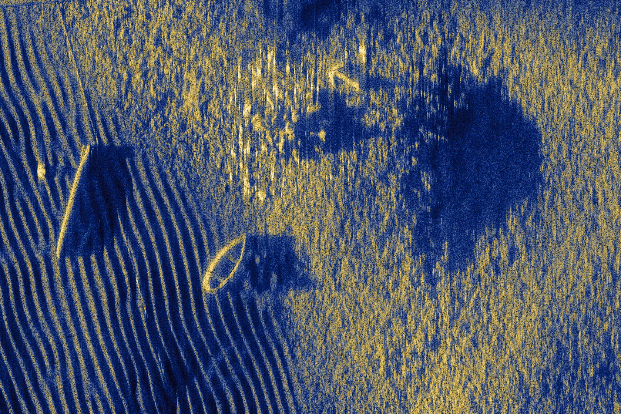
Synthetic aperture sonar image of the whole scene formed with the estimated navigation: rippled sand over the near half, a pipeline crossing the scene, and a boat, rocks and other objects in the far half. Sensor navigation Estimated navigation
The whole scene, 70 m of ground range from beneath the vehicle by 50 m of track, reduced from 3500 by 2500 pixels. The coefficient of variation of the image magnitude is 1.54 with the sensor navigation, 1.69 with the estimated navigation and 1.72 with the true track.

Scope

Limitations

Simulated data
The record is a simulation without receiver noise, so the correlation over the seabed is higher than a sea trial would give.
Straight track
The true motion is zero in sway and heave, so the result bounds the motion the estimator invents and does not measure how well it recovers motion that is present.
Degrees of freedom
Surge and attitude are taken from the navigation, which is exact in this record; on a vehicle they come from a Doppler velocity log and an inertial unit with their own errors.
Seabed model
The motion model and the image both assume a horizontal seabed, while the seabed of the scene rises by about 7 m across the swath and the wreck stands about 17 m above it.
Receiver rows
One of the two receiver rows is used, so the record's interferometric information is not.
Simulated vehicle
The vehicle result is one scene with one draw of the sensor errors and no receiver noise, so it does not give the spread of the estimate over seabeds or sensors.

Sources

References

  1. B. Thomas and A. Hunter, "Simulated Interferometric Synthetic Aperture Sonar (InSAS) Data of the SS Thistlegorm Wreck," University of Bath Research Data Archive, 2023. doi:10.15125/BATH-01219. Licensed under CC BY 4.0.
  2. B. W. Thomas and A. J. Hunter, "Interferometric synthetic aperture sonar large scale simulated data benchmark of a ship wreck," Electronics Letters, vol. 59, no. 10, e12810, 2023. doi:10.1049/ell2.12810.
  3. I. D. Gerg, D. C. Brown, S. G. Wagner, D. Cook, B. N. O'Donnell, T. Benson and T. C. Montgomery, "GPU Acceleration for Synthetic Aperture Sonar Image Reconstruction," 2021. arXiv:2101.05888.
  4. B. Jalving, K. Gade, K. Svartveit, A. Willumsen and R. Sørhagen, "DVL Velocity Aiding in the HUGIN 1000 Integrated Inertial Navigation System," Modeling, Identification and Control, vol. 25, no. 4, pp. 223-236, 2004. doi:10.4173/mic.2004.4.2.
Next: image formation, the processing chain used on this page, or the surface of focus, why the wreck is displaced in these images.