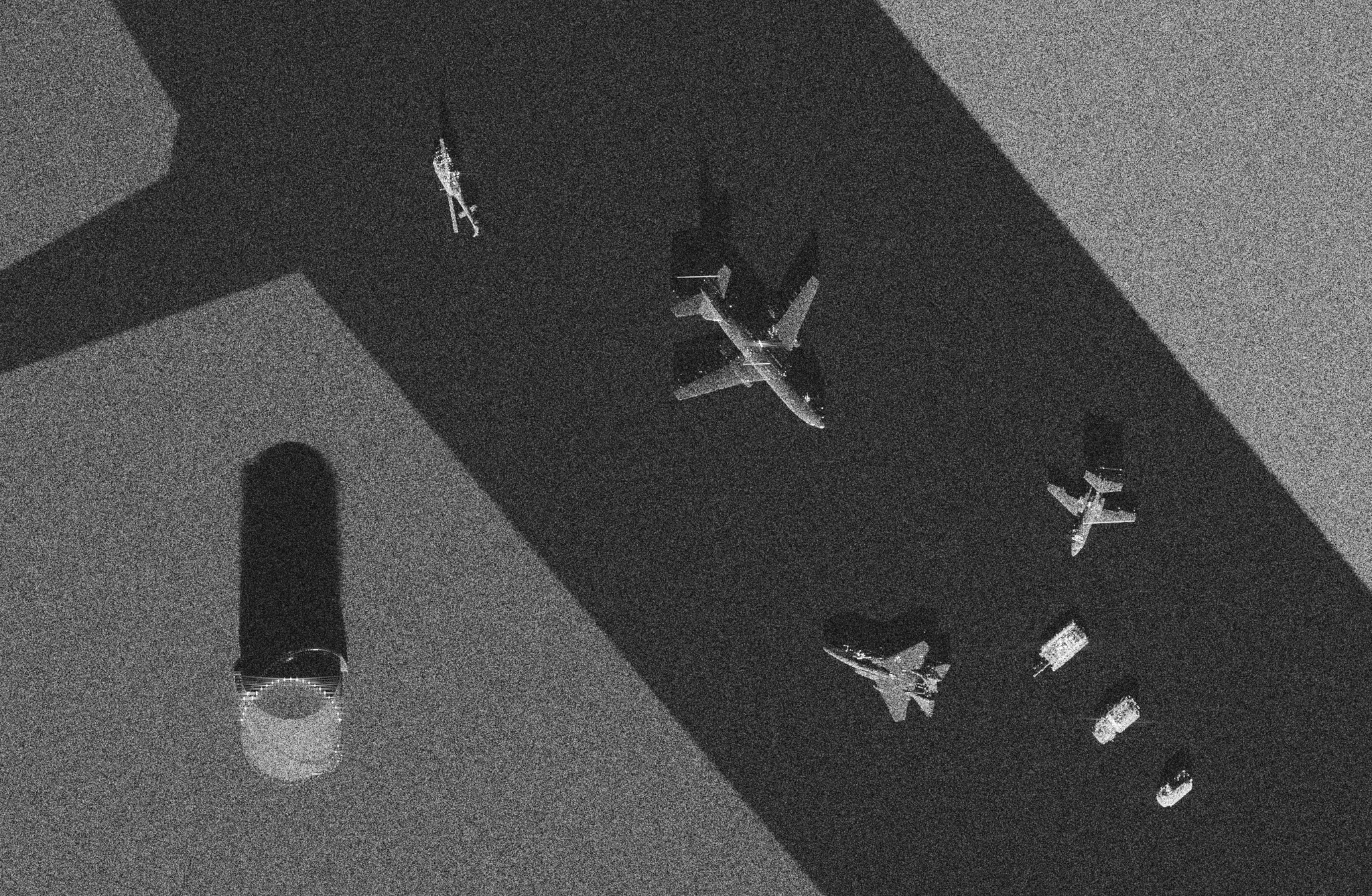
An airfield apron imaged as synthetic aperture radar

ApertureLab's simulator and beamformer are not specific to sound in water. Given a radar's wavelength, bandwidth, antenna and flight geometry, the same scene description, scattering engine and back-projection beamformer form a synthetic aperture radar (SAR) image. The image on this page is an airfield apron seen by a Ku-band airborne radar at 0.1 m resolution from a slant range of 3.1 km. The radar parameters and the geometry are those of a publicly released Sandia MiniSAR image; the levels of the pavement, the soil and the receiver noise were measured on that image.

Scene

Height map and SAR image
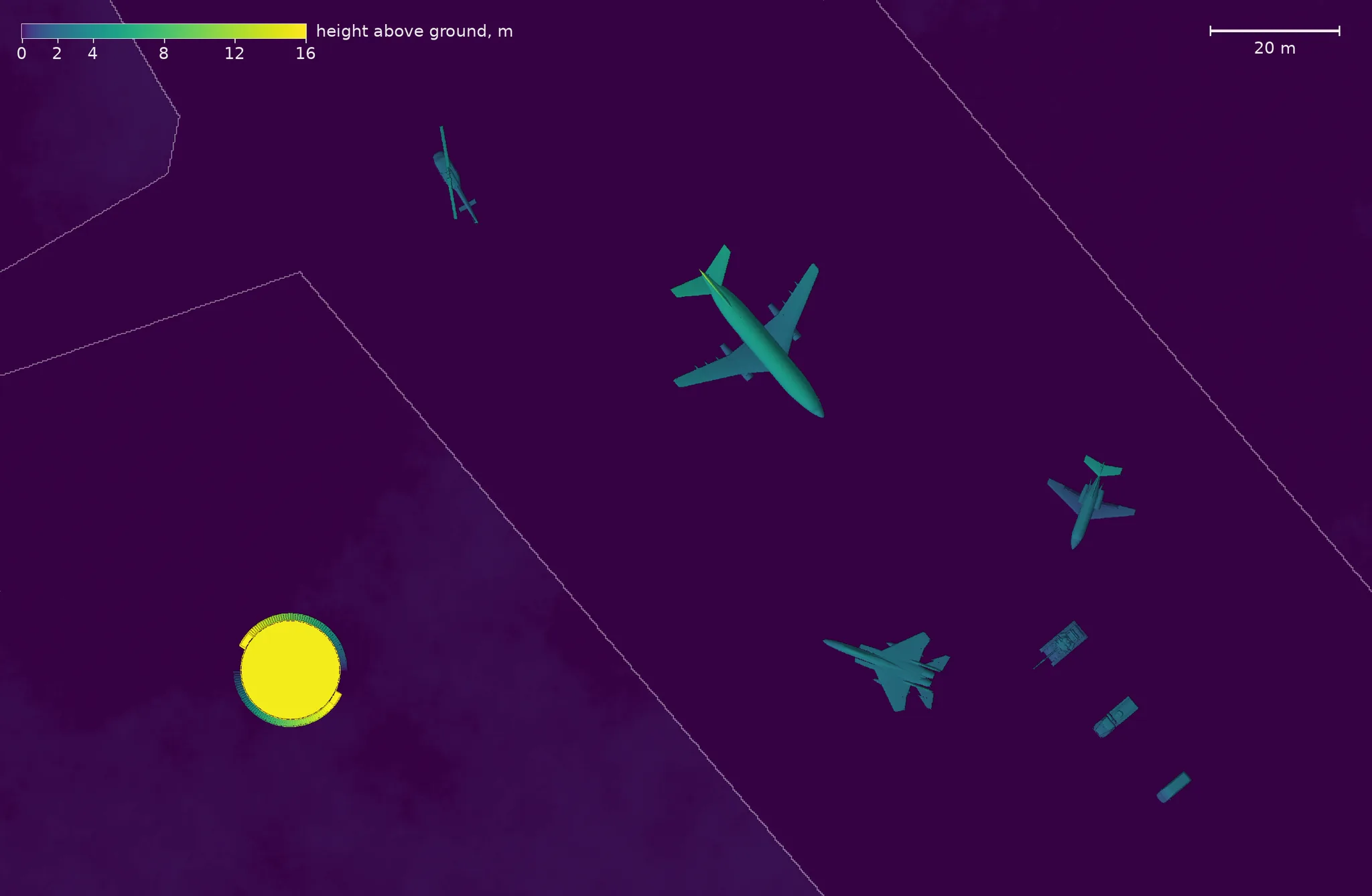
Top-down height map of the scene in color. A paved apron crosses the frame diagonally between two areas of bare soil, its edges drawn as thin lines. On the apron stand an airliner, two smaller aircraft, a helicopter and a row of three vehicles; a round storage tank 15 meters tall stands on the soil at the lower left. A color bar runs from 0 to 16 meters and a scale bar marks 20 meters.
Height map of the scene on the pixel grid of the image below. Color is height above the ground on a square-root scale; the thin lines are the edges of the paved apron, with bare soil on either side. The scene holds three aircraft, a helicopter, three vehicles and a storage tank 15 m tall. The footprint is 212.5 m in azimuth by 138.7 m in ground range.
Grayscale synthetic aperture radar image of the same footprint. The apron is a dark diagonal band between brighter soil. Each aircraft and vehicle appears as a bright speckled outline with sharp glints, displaced toward the bottom of the frame, with a darker shadow extending toward the top. The storage tank's roof appears as a bright disc below a long shadow.
The simulated SAR image of the same footprint. Azimuth runs left to right and ground range increases up the page; the radar is below the bottom edge. Pixels are 0.0847 m. The shadows are not black because the image carries a receiver noise floor 12.9 dB below the level of the soil at the lower left. The figure enlarges when selected.

Instrument

Radar and collection geometry

The radar is modeled on the Sandia MiniSAR, a Ku-band airborne system. The center frequency, range, grazing angle, platform speed and pixel spacing are read from the header of the reference image, and the simulated collection has the following parameters.

Frequency
The center frequency is 16.8 GHz (a wavelength of 17.8 mm) on one channel with horizontal polarization on transmit and receive.
Bandwidth
The pulse spans 2.5 GHz and is sampled at 3.125 GHz, which gives 0.086 m of slant-range resolution after the Hann-weighted matched filter.
Platform
The aircraft flies straight and level at 65.7 m/s, 1584 m above the ground, looking to the side.
Range and grazing angle
The scene center lies at 3074 m slant range and is viewed at a grazing angle of 31.0 degrees.
Synthetic aperture
Every pixel is integrated over 7.2 degrees of azimuth, 387 m of track at the scene center, with Taylor weighting.
Pulses
The radar transmits every 0.08 m of track, 7763 pulses over 621 m.
Image formation
Time-domain back-projection onto the ground plane forms 2510 by 1639 pixels of 0.0847 m.
Measured resolution
A trihedral reflector in the far corner of the image measures 0.101 m in azimuth and 0.103 m in ground range at the half-power points; the header of the reference image states 0.1016 m for both.
Scattering
The ground is 200 point scatterers per square meter with one level for each ground class. The objects are Kirchhoff facets with an 18 mm edge and add double-bounce returns off the pavement and off their own flat faces. The layout of the objects is invented, and their returns are not calibrated against measured radar cross sections.

Mode

Spotlight and stripmap collection

The MiniSAR forms its 0.1 m images in spotlight mode. The antenna is steered to hold one patch of ground in the beam while the aircraft flies past, so the patch is observed over a wider angle than a fixed beam of that antenna would allow, and the azimuth resolution follows from the angle rather than from the antenna length.

A synthetic aperture sonar is collected in stripmap mode instead. The beam stays broadside, the vehicle images a continuous swath along its track, and the along-track resolution is half the element length at every range. A sonar element a few centimeters long already has a beam wide enough for centimeter resolution, so nothing is gained by steering it, and the survey calls for the continuous swath.

The simulated collection reproduces the spotlight aperture with a fixed beam. The antenna is shortened to 0.09 m, so that its broadside beam spans the 7.2 degree aperture, and the track is extended so that every pixel is observed over that full angle. The resolution and the pixel spacing are those of the spotlight image. The difference is that each pixel is viewed about its own broadside rather than about the scene center, which changes the viewing direction by up to 2 degrees at the azimuth edges of this scene.

The aircraft and helicopter models are by mgg8 of the Aviation Gazetteer and are in the public domain (CC0). Four models are used under CC BY 4.0, each converted to a triangle mesh in meters and scaled to its true size: Process Storage Tank by Deepak Singh, Ural ATZ-5-4320 Fuel truck by Basic Hsu, Mercedes-Benz Sprinter by Savelliy 07 and T-72M4CZ Variation by Elianiq.

Next: Kirchhoff facets, the scattering model of the objects in this scene, or the differences between SAS and SAR.